Statistical analysis of project estimates, or why correct estimates are always exceeded
In my work, I constantly have to make assessments for projects, tasks and work that have yet to be completed, and therefore it is impossible to measure them accurately. Recently, one of the major clients of Accenture turned to our company with a request to help in developing a more systematic method for preparing such estimates. The project did not happen, but the materials that I collected turned out to be extremely useful for myself. I could understand why, in spite of the planning of projects according to carefully verified estimates, people almost always exceed the budget. I realized that by guaranteeing that they fit into the budget with a 95% probability, the contractors guarantee that with a 95% probability they don’t need that much time and money. Below I have described my calculations that you might also be interested in.
The first thing I did when I joined this project was to try to formulate the essence of the problem, that is, the task that I want to solve. In almost all the projects in which I was involved, the plan was based on precise estimates of individual tasks, on specific numbers indicated as duration, effort or cost of the task. Only a few projects used the PERT method, determining, in addition to the most expected costs, also optimistic and pessimistic estimates, but even in this case, the overall assessment of the project was one particular number. I understood that in reality the actual costs will always be more or less than the initial estimate, and the probability of exact match tends to zero. I was sure that any allocated budget would be either overexpenditures or not sufficient. Our potential client and I personally wanted to be able to determine the probability of fitting into a particular budget, i.e. on the one hand, to avoid a situation where money runs out in the middle of a project, and on the other hand, to avoid a situation where there is extra money left that is simply “mastered” without already bringing additional profits to the business.
And then I was lucky: our company, being one of the world's largest service providers in the field of outsourcing, has huge amounts of data on completed projects, and I was able to quickly get a large sample of data from one of the Russian projects. I received estimates and actual costs for several thousand bids with typical labor costs from 1 to 50 hours. After simple manipulations in Excel, I received the desired distribution (Fig. 1). On the histogram, the number of applications is postponed vertically, and the amount of actual costs relative to the projected ones is horizontal. For example, if the actual costs coincide with the estimate, then on the histogram such an application will increase by one the bar at point 1. If the actual costs are half a day in the assessment of two days, then the application will fall to a point of 0.25.
Fig.1. Distribution of actual costs in a single project

')
Here is what I saw when analyzing the resulting graph:
Firstly, it turned out that our employees make very realistic assessments, i.e. indicate those costs, the probability of which is maximum (in the graph, this point is marked in green). If our expert says that some task will take 12 hours, then the probability that the task will take exactly 12 hours is slightly higher than the probability that the real costs will be 11 or 13 hours, and much higher than the costs that will be equal to 6 or 24 hours .
Secondly, when I calculated the average costs for all applications, I found that the arithmetic mean turned out to be noticeably larger than the initial estimates. In the first year of the project, the average cost exceeded the initial estimate by 50%, then the difference was reduced to 30%, but it did not disappear anywhere. This strange at first glance fact was found a simple explanation. We can err on the side of reducing costs, not more than on the initial estimate (the amount of costs cannot be negative), and we have almost no limits on exceeding the mark, and the actual costs can exceed the mark by two, three, four or even ten times. Examples, unfortunately, are available. As a result, errors in the direction of increasing costs outweigh the errors in the direction of decreasing, and on average real costs turn out to be more than the most plausible and probable estimates. In the language of statistics, it turns out that the distribution of actual costs is asymmetrical, and the expectation is greater than the distribution mode.
The next important observation is the behavior of people who ensure that they fit into the promised costs. In order to be sure of this, they subscribe to that cost estimate, the risk to exceed which is no more than 5-10%. And this means that the probability that the real costs will be less than the promised - 90-95%, and judging by the distribution obtained - will exceed 2-3 times. It turns out that guaranteed compliance with the budget and deadlines results in a 2-3 fold increase in the budget and deadlines, i.e. strict control of deadlines and budgets without regard for their adequacy and realism guarantees a fall in overall efficiency .
In order to fight this effect, some customers and executives require specifying the most likely cost estimates as targeted, and agree to forgive the possible overshooting of estimates in the context of contingency reserves. Unfortunately, the size of such reserves rarely exceeds 20%, and as I wrote above, the costs of individual tasks on average exceed the plausible estimates by 30-50%. Within the framework of a large project, errors in individual tasks can compensate for each other, but, nevertheless, over time, errors accumulate and lead to a guaranteed excess of the target budget .
To overcome this detrimental effect, you can use one of two methods: you can try to calculate the correction factor to the sum of plausible estimates, or use the PERT method developed in the 50s of the last century based on the ideas of Henry Ford and Frederick Taylor. The first method is simpler, but the second one allows not only to get a realistic estimate, but also to understand what is the distribution of possible values of actual costs.
***
In order to calculate a realistic estimate based on the most plausible, using a correction factor, this coefficient must first be calculated. To do this, you need to take at least 20-40 completed tasks and calculate the average ratio of actual costs to the original estimate. If the size of the estimates differ by more than two or three times, then it makes sense to determine two, three or even more coefficients for problems of different sizes. In the data I used, the correction factor for problems with a rating of less than 2 hours-hour turned out to be three times the coefficient for problems with a rating of 12 to 24 hours.
After the set of correction factors has been obtained, it is necessary to multiply each plausible estimate by the corresponding correction factor, and sum the resulting works. The result will be a realistic estimate of project costs, for which the risk of the supplier to exceed the budget is equal to the risk of the customer paying extra.
The disadvantage of this method is the strong dependence of the result on the accuracy of the calculation of the correction factor, so most Agile methodologies using this method require clarification of the correction factor after each iteration or release. In addition, these methodologies stimulate to break work into tasks of approximately the same size, which makes it possible to manage with just one coefficient.
***
The PERT method, in contrast to the previous method, does not use any predetermined coefficients and uses several estimates for each task to calculate a realistic estimate for the entire project.
In order to calculate a realistic assessment of the project using the PERT methodology, it is necessary to specify three estimates for each task: the most plausible estimate obtained in the usual way, optimistic — estimating the minimum costs if we overestimate the complexity of the task, and pessimistic — estimating the maximum costs that may be required to complete the task. After that, a realistic assessment of a separate task is determined by the formula below. The costs for the project as a whole are estimated by summing up the realistic estimates for each task.


Where
μ - a realistic estimate of the cost of the project or release as a whole,
n is the number of tasks in a project or release,
μ i - realistic cost estimate for task i,
O i - an optimistic estimate of the cost of task i,
E i - the most plausible cost estimate for task i,
P i - pessimistic cost estimate for task i
It is important to pay attention to another feature of the data - the probability of making a mistake two times downward turned out to be equal to the probability of making a mistake two times upwards. Those. the distribution of the relative error (in contrast to the absolute error) turned out to be symmetric. Accordingly, the ratio of a realistic estimate to an optimistic one should be minimally different or equal to the ratio of the pessimistic estimate of costs to a realistic estimate.

If this is not the case, then it makes sense to check the correctness of optimistic and pessimistic assessments.
***
To determine the necessary reserves for unforeseen needs, it is necessary to calculate the interval of possible costs for a given estimate (see Figure 2). If the initial estimate for the task was 16 hours, then with a 50% probability we can say that the actual costs will be in the range from 15 to 24 hours, and with a 95% probability it could only be said that the costs will be ranging from 3 to 56 h-hours.
Figure 2. Confidence Interval
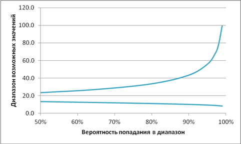
The most typical is to use the range with a probability of 90%. In this case, the probabilities that the cost value exceeds the pessimistic estimate, and that the costs will be less than the optimistic estimate, are assumed to be equal to 5%. The likelihood that actual costs fall within the range between optimistic and pessimistic estimates is 90%.
Obtaining the probability distribution of actual costs for the release and the project is possible using optimistic and pessimistic estimates obtained in the PERT method. The method itself for obtaining a range of possible values suggests simply adding up optimistic and pessimistic estimates, but the simplest modeling shows that this is incorrect. Pessimistic assessment of the project is less than the sum of estimates, and optimistic - more. The range with a probability of 90% is less than the simple sum of the ranges for individual tasks.
There is no exact formula for calculating the range of randomly distributed values we need, but a good approximation is given by the following formula, which suggests that the spread of possible cost values increases in proportion to the square root of the number of tasks in a project or release:


Accordingly, the more detailed we break up a large project and think more about each individual task, the more accurate we can give an estimate. For example, if you take a large integration project implementation, the labor costs for which can be 50,000 h-days, then breaking the plan into 1,000 tasks we can theoretically get an error of less than 800 h-days or less than 2%. The graph of the theoretical dependence of the cost variation depending on the detail of the plan is shown in Fig.3.
Fig.3. The theoretical dependence of the accuracy of cost estimation depending on the number of subtasks in the plan:
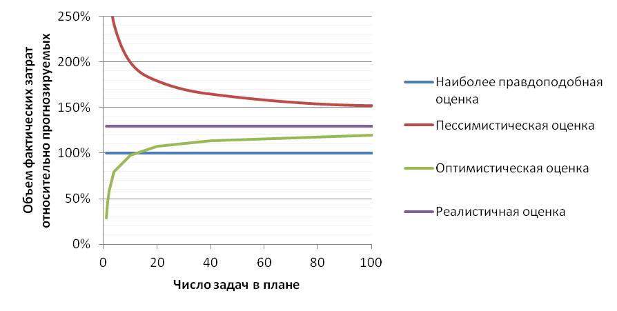
Unfortunately, in real life there are a number of restrictions that do not allow to achieve such accuracy, and the most significant is that the requirements and composition of the tasks performed may change during the course of the project. For most companies, 10-30% of tasks are typical for a loss, so no matter how detailed the plan is, a mistake in the initial estimates is inevitable.
Summarizing the findings, I was able to understand the following. Using the amount of the most plausible cost estimates for evaluating a large project, we are guaranteed to underestimate the estimate, summing up the pessimistic estimates - it is guaranteed to be overestimated. In order to obtain a realistic estimate, it is necessary to use a previously calculated correction factor or a PERT estimation method. Using the estimates in the PERT methodology, we can also get a range of costs, about which we can say that the actual costs will fall into it with a probability of 90% and in which there are no excess reserves. And by detailing the project plan and carefully evaluating each task, it is possible to significantly reduce this range, eventually reaching the required amount of reserves.
The first thing I did when I joined this project was to try to formulate the essence of the problem, that is, the task that I want to solve. In almost all the projects in which I was involved, the plan was based on precise estimates of individual tasks, on specific numbers indicated as duration, effort or cost of the task. Only a few projects used the PERT method, determining, in addition to the most expected costs, also optimistic and pessimistic estimates, but even in this case, the overall assessment of the project was one particular number. I understood that in reality the actual costs will always be more or less than the initial estimate, and the probability of exact match tends to zero. I was sure that any allocated budget would be either overexpenditures or not sufficient. Our potential client and I personally wanted to be able to determine the probability of fitting into a particular budget, i.e. on the one hand, to avoid a situation where money runs out in the middle of a project, and on the other hand, to avoid a situation where there is extra money left that is simply “mastered” without already bringing additional profits to the business.
And then I was lucky: our company, being one of the world's largest service providers in the field of outsourcing, has huge amounts of data on completed projects, and I was able to quickly get a large sample of data from one of the Russian projects. I received estimates and actual costs for several thousand bids with typical labor costs from 1 to 50 hours. After simple manipulations in Excel, I received the desired distribution (Fig. 1). On the histogram, the number of applications is postponed vertically, and the amount of actual costs relative to the projected ones is horizontal. For example, if the actual costs coincide with the estimate, then on the histogram such an application will increase by one the bar at point 1. If the actual costs are half a day in the assessment of two days, then the application will fall to a point of 0.25.
Fig.1. Distribution of actual costs in a single project
')
Here is what I saw when analyzing the resulting graph:
Firstly, it turned out that our employees make very realistic assessments, i.e. indicate those costs, the probability of which is maximum (in the graph, this point is marked in green). If our expert says that some task will take 12 hours, then the probability that the task will take exactly 12 hours is slightly higher than the probability that the real costs will be 11 or 13 hours, and much higher than the costs that will be equal to 6 or 24 hours .
Secondly, when I calculated the average costs for all applications, I found that the arithmetic mean turned out to be noticeably larger than the initial estimates. In the first year of the project, the average cost exceeded the initial estimate by 50%, then the difference was reduced to 30%, but it did not disappear anywhere. This strange at first glance fact was found a simple explanation. We can err on the side of reducing costs, not more than on the initial estimate (the amount of costs cannot be negative), and we have almost no limits on exceeding the mark, and the actual costs can exceed the mark by two, three, four or even ten times. Examples, unfortunately, are available. As a result, errors in the direction of increasing costs outweigh the errors in the direction of decreasing, and on average real costs turn out to be more than the most plausible and probable estimates. In the language of statistics, it turns out that the distribution of actual costs is asymmetrical, and the expectation is greater than the distribution mode.
The next important observation is the behavior of people who ensure that they fit into the promised costs. In order to be sure of this, they subscribe to that cost estimate, the risk to exceed which is no more than 5-10%. And this means that the probability that the real costs will be less than the promised - 90-95%, and judging by the distribution obtained - will exceed 2-3 times. It turns out that guaranteed compliance with the budget and deadlines results in a 2-3 fold increase in the budget and deadlines, i.e. strict control of deadlines and budgets without regard for their adequacy and realism guarantees a fall in overall efficiency .
In order to fight this effect, some customers and executives require specifying the most likely cost estimates as targeted, and agree to forgive the possible overshooting of estimates in the context of contingency reserves. Unfortunately, the size of such reserves rarely exceeds 20%, and as I wrote above, the costs of individual tasks on average exceed the plausible estimates by 30-50%. Within the framework of a large project, errors in individual tasks can compensate for each other, but, nevertheless, over time, errors accumulate and lead to a guaranteed excess of the target budget .
To overcome this detrimental effect, you can use one of two methods: you can try to calculate the correction factor to the sum of plausible estimates, or use the PERT method developed in the 50s of the last century based on the ideas of Henry Ford and Frederick Taylor. The first method is simpler, but the second one allows not only to get a realistic estimate, but also to understand what is the distribution of possible values of actual costs.
***
In order to calculate a realistic estimate based on the most plausible, using a correction factor, this coefficient must first be calculated. To do this, you need to take at least 20-40 completed tasks and calculate the average ratio of actual costs to the original estimate. If the size of the estimates differ by more than two or three times, then it makes sense to determine two, three or even more coefficients for problems of different sizes. In the data I used, the correction factor for problems with a rating of less than 2 hours-hour turned out to be three times the coefficient for problems with a rating of 12 to 24 hours.
After the set of correction factors has been obtained, it is necessary to multiply each plausible estimate by the corresponding correction factor, and sum the resulting works. The result will be a realistic estimate of project costs, for which the risk of the supplier to exceed the budget is equal to the risk of the customer paying extra.
The disadvantage of this method is the strong dependence of the result on the accuracy of the calculation of the correction factor, so most Agile methodologies using this method require clarification of the correction factor after each iteration or release. In addition, these methodologies stimulate to break work into tasks of approximately the same size, which makes it possible to manage with just one coefficient.
***
The PERT method, in contrast to the previous method, does not use any predetermined coefficients and uses several estimates for each task to calculate a realistic estimate for the entire project.
In order to calculate a realistic assessment of the project using the PERT methodology, it is necessary to specify three estimates for each task: the most plausible estimate obtained in the usual way, optimistic — estimating the minimum costs if we overestimate the complexity of the task, and pessimistic — estimating the maximum costs that may be required to complete the task. After that, a realistic assessment of a separate task is determined by the formula below. The costs for the project as a whole are estimated by summing up the realistic estimates for each task.
Where
μ - a realistic estimate of the cost of the project or release as a whole,
n is the number of tasks in a project or release,
μ i - realistic cost estimate for task i,
O i - an optimistic estimate of the cost of task i,
E i - the most plausible cost estimate for task i,
P i - pessimistic cost estimate for task i
It is important to pay attention to another feature of the data - the probability of making a mistake two times downward turned out to be equal to the probability of making a mistake two times upwards. Those. the distribution of the relative error (in contrast to the absolute error) turned out to be symmetric. Accordingly, the ratio of a realistic estimate to an optimistic one should be minimally different or equal to the ratio of the pessimistic estimate of costs to a realistic estimate.
If this is not the case, then it makes sense to check the correctness of optimistic and pessimistic assessments.
***
To determine the necessary reserves for unforeseen needs, it is necessary to calculate the interval of possible costs for a given estimate (see Figure 2). If the initial estimate for the task was 16 hours, then with a 50% probability we can say that the actual costs will be in the range from 15 to 24 hours, and with a 95% probability it could only be said that the costs will be ranging from 3 to 56 h-hours.
Figure 2. Confidence Interval
The most typical is to use the range with a probability of 90%. In this case, the probabilities that the cost value exceeds the pessimistic estimate, and that the costs will be less than the optimistic estimate, are assumed to be equal to 5%. The likelihood that actual costs fall within the range between optimistic and pessimistic estimates is 90%.
Obtaining the probability distribution of actual costs for the release and the project is possible using optimistic and pessimistic estimates obtained in the PERT method. The method itself for obtaining a range of possible values suggests simply adding up optimistic and pessimistic estimates, but the simplest modeling shows that this is incorrect. Pessimistic assessment of the project is less than the sum of estimates, and optimistic - more. The range with a probability of 90% is less than the simple sum of the ranges for individual tasks.
There is no exact formula for calculating the range of randomly distributed values we need, but a good approximation is given by the following formula, which suggests that the spread of possible cost values increases in proportion to the square root of the number of tasks in a project or release:
Accordingly, the more detailed we break up a large project and think more about each individual task, the more accurate we can give an estimate. For example, if you take a large integration project implementation, the labor costs for which can be 50,000 h-days, then breaking the plan into 1,000 tasks we can theoretically get an error of less than 800 h-days or less than 2%. The graph of the theoretical dependence of the cost variation depending on the detail of the plan is shown in Fig.3.
Fig.3. The theoretical dependence of the accuracy of cost estimation depending on the number of subtasks in the plan:
Unfortunately, in real life there are a number of restrictions that do not allow to achieve such accuracy, and the most significant is that the requirements and composition of the tasks performed may change during the course of the project. For most companies, 10-30% of tasks are typical for a loss, so no matter how detailed the plan is, a mistake in the initial estimates is inevitable.
Summarizing the findings, I was able to understand the following. Using the amount of the most plausible cost estimates for evaluating a large project, we are guaranteed to underestimate the estimate, summing up the pessimistic estimates - it is guaranteed to be overestimated. In order to obtain a realistic estimate, it is necessary to use a previously calculated correction factor or a PERT estimation method. Using the estimates in the PERT methodology, we can also get a range of costs, about which we can say that the actual costs will fall into it with a probability of 90% and in which there are no excess reserves. And by detailing the project plan and carefully evaluating each task, it is possible to significantly reduce this range, eventually reaching the required amount of reserves.
Source: https://habr.com/ru/post/143116/
All Articles