Perlin Noise
Good day. I bring to your attention the translation of the article about Perlin noise ( this one ). Links to this article already flashed on Habré ( here ), but I did not get a translation of the article. So I hope someone can be useful.
Many people had to use random number generator in programs to create unpredictability, to make the movement and behavior of objects more natural or generate textures. Random number generators, of course, have their own uses, but sometimes their output can be too “hard” to seem natural. In this article, we present a feature that has a very wide range of applications, more than I could think, but mostly wherever you need something to look natural. In addition, the output can be easily customized to your needs.
If you look at many things in nature, you will notice that they are fractal. They have different levels of detail. A typical example is the outline of a mountain range. It contains significant differences in altitude (mountains), medium variations (hills), small variations (boulders), tiny variations (stones), and so on. Look at anything: spreading grass spots on the field, waves in the sea, the movement of ants, the movement of the branches of a tree, patterns of marble, wind. All these phenomena lend themselves to the same pattern, in large and small variations. The Perlin noise function recreates this by simply folding the noise functions at various scales.
')
To create the Perlin noise function, you need two things, the noise function and the interpolation function.
The noise function is essentially a random number generator sample. It takes an integer as a parameter, and returns a random number based on this parameter. If you pass the same parameter twice, it will give the same number twice. It is very important that she behaves in this way, otherwise there will be no sense from her.
Here is a graph showing an example of the noise function. A random value from 0 to 1 is assigned to each point on the X axis.
By smooth interpolation between values, we can define a continuous function that takes a non-integer as a parameter.
Different ways of interpolating values will be later in this article.
Before I go any further, let me determine what I mean by amplitude and frequency. If you studied physics, you could well meet the concept of amplitude and frequency as applied to a sine-wave.
(amplitude - amplitude, wavelength - wavelength, frequency - frequency)
Wavelength is the distance from one vertex to another. The amplitude is the height of the wave. Frequency is defined as 1 / (wavelength).
On the graph of this noise function, for example, red dots indicate random values determined from the dimension of the function.
In this case, the amplitude is the difference between the minimum and maximum values that the function may have. The wavelength is the distance from one red spot to another. Again, the frequency is defined as 1 / (wavelength).
Now, if you take a lot of such smooth functions, with different frequency and amplitude, you can add them all together to create a well-noisy function. This is the Perlin noise function.
Take the following noise function
Match them together and that's what you get in the end.
You can see that this feature has large, medium and small variations. You can even imagine that it looks a bit like a mountain range. In fact, many computer landscapes are made using this method. Of course they use the 2D noise I received at the moment.
You, of course, can do the same for two dimensions. Some noise functions in 2D

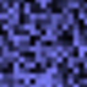

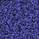

Putting all these functions together we get a noise picture.

When you add these noise functions together, you may wonder what exactly the amplitude and frequency is used for each of them. In the one-dimensional example, the frequency and half amplitude are used twice for each subsequent added noise function. This is quite common. Thus, in fact, many people do not even consider using the rest. However, you can create noise Perlin functions with different characteristics and using different frequencies and amplitudes at each step. For example, to create smooth hills, you can use the Perlin noise function with large amplitudes at low frequencies, and very small amplitudes at high frequencies. Or you could make a flat, but very rocky plane by choosing small amplitudes for low frequencies.
To explain it more simply, and to avoid repeating the words “amplitude” and “frequency” all the time, a single number is used to determine each amplitude and each frequency. This value is called persistence. There is some uncertainty about its exact meaning. This term was originally coined by Mandelbrot, one of those who are behind the discovery of fractals. He identified noise with a lot of high frequencies with low durability. My friend Matt also came up with the concept of perseverance, but determined it the other way around. Honestly, I prefer the definition of Matt.
Sorry, Mandelbrot.
Thus, our definition of perseverance is as follows:
Where i is the i-th noise function added.
To illustrate the effect of perseverance on the output of Perlin noise, take a look at the diagrams below.
They show the noise component of the function that is added, the effect of storing the value, and, as a consequence, the Perlin noise function.
frequencies: 1, 2, 4, 8, 16, 32


 =
= 
Amplitudes: 1, 1/4, 1/16, 1/64, 1/256, 1/1024
frequencies: 1, 2, 4, 8, 16, 32


 =
= 
Amplitudes: 1, 1/2, 1/4, 1/8, 1/16, 1/32
frequencies: 1, 2, 4, 8, 16, 32


 =
= 
Amplitudes: 1, 1 / 1.414, 1/2, 1 / 2.828, 1/4, 1 / 5.656
frequencies: 1, 2, 4, 8, 16, 32


 =
= 
Amplitudes: 1, 1, 1, 1, 1, 1
Each subsequent noise function added is called an octave. The reason for this is that each noise function has a frequency twice as large as the previous one. In music, the octave also has this property.
How many octaves you will add is entirely up to you. You can add as many or as few as you want. However, let me give you some tips. If you use the Perlin noise function to render an image to the screen, a moment will come when the octave may have a frequency too high to be displayed. There simply may not be enough pixels on the screen to reproduce all the fine details at a very high noise function. Some Perlin noise implementations are automatically added up from noise functions until the screen resolution limits (or other environment) are reached.
In addition, it is reasonable to stop when adding a noise function, when their amplitude becomes too small to influence the result. When this happens will depend on the level of endurance, the overall amplitude of the Perlin function and a bit of the screen resolution (or something else).
What are we looking for in the noise function? Essentially - a random number generator. However, unlike other random number generators that you encounter in programs that give you different random numbers each time you call them, these noise functions produce a random number calculated from one or more parameters. That is, each time you enter the same number, the noise function will respond with the same number as before for that number. But by entering another number, it will return another number.
Well, I don't know much about random number generators, so I started searching, and here is one I found. He looked pretty good. It returns floating-point numbers from -1.0 to 1.0.
Now, you probably want several different random number generators, so I suggest making a few copies of the code above, but using slightly different numbers. These big creepy-looking numbers are all prime numbers, so you could just use some other prime numbers of the same size. So in order to make it easy for you to find random numbers, I wrote a small program to the list of prime numbers for you. You can give her a starting and ending number, and she will find all the prime numbers between them. Source code is also included, so you can easily include it in your programs to create a random prime number ( program and code ).
(in order not to strain the resource I spread the code, here it is completely, because there is not a lot of it )
After creating your noise function, you need to smooth out the values it returns. Again, you can choose any method you like, but some look better than others. The standard interpolation functions have three inputs, a, b, the values for interpolation between them, and x, which takes values from 0 to 1. The interpolation function returns a value between a and b depending on the value of x. If x is 0, then a is returned, and when x = 1, then b is returned. If x is between 0 and 1, then it returns a value between a and b.
It looks awful, like cheap "plasma" that many use to create landscapes. This is a simple algorithm, though, and I suppose it would be excusable if you tried to make Perlin noise in real time.

This method gives a smoother curve than linear interpolation. This is clearly the best result and is well worth the effort if you can afford a very small loss in speed.

This method gives very smooth results, but you pay for it in speed. To be honest, I'm not sure that this will give much better results than the cosine interpolation, but here it is in any case at your discretion. This is a little more complicated, so be careful. If earlier, for the interpolation function there were three inputs, the cubic interpolation takes five. Instead of a and b, now you need v0, v1, v2 and v3, along with x, as before.

v0 = point to a
v1 = point a
v2 = point b
v3 = point after b

In addition to interpolation, you can also smooth out the output of the noise function to make it less random looking, as well as less area in the 2D and 3D versions. Smoothing will do more than you expect, and everyone who has written a smoothing filter or a fire algorithm should already be familiar with this process. Instead of just taking the values of the noise function in one of the coordinates, you can take the average of this value and the value in the next coordinates. If this is not clear, take a look at the pseudocode below.
In the small diagram, the differences between the smoothed noise function and the same noise function without smoothing are illustrated.
You can see that the smooth noise function is smoothed, never reaches the extremes of a smooth noise function and the frequency is about two times less. There is little point in smoothing out the 1-dimensional noise, as this is really the only effect. Smoothing becomes more useful in 2 or three dimensions, where the effect is to reduce the squareness of the noise.
Unfortunately, it also reduces the contrast. The smoother you make it, obviously, the noise will be flatter.


Now you know everything, so it's time to put together everything you learned and create the Perlin noise function. Remember that these are just a few additions of the interpolations of the noise function. Thus, Perlin noise is just a function. You pass one or more parameters, and it responds with a number.
So, here is a simple 1-dimensional function of Perlin. The main part of the function of the Pearl is a cycle. Each iteration of the loop adds another double octave. Each iteration causes different noise functions, denoted Noise i . Now you don’t actually need to write a lot of noise functions, one for each octave, as you would expect in pseudocode. Since all the noise functions are almost the same, except for the values of these three large primes, you can save the same code, but simply use a different set of prime numbers for each.
Now you can easily apply the same code to create 2 or more dimensional Perlin noise functions.
At the end of the original article there are additional materials, who will be interested, I think it will not be difficult to proceed.
References:
Actually the article itself .
Ken Perlin website
ps: Dear minus, but to motivate the minus is not accepted?
Many people had to use random number generator in programs to create unpredictability, to make the movement and behavior of objects more natural or generate textures. Random number generators, of course, have their own uses, but sometimes their output can be too “hard” to seem natural. In this article, we present a feature that has a very wide range of applications, more than I could think, but mostly wherever you need something to look natural. In addition, the output can be easily customized to your needs.
If you look at many things in nature, you will notice that they are fractal. They have different levels of detail. A typical example is the outline of a mountain range. It contains significant differences in altitude (mountains), medium variations (hills), small variations (boulders), tiny variations (stones), and so on. Look at anything: spreading grass spots on the field, waves in the sea, the movement of ants, the movement of the branches of a tree, patterns of marble, wind. All these phenomena lend themselves to the same pattern, in large and small variations. The Perlin noise function recreates this by simply folding the noise functions at various scales.
')
To create the Perlin noise function, you need two things, the noise function and the interpolation function.
Noise function
The noise function is essentially a random number generator sample. It takes an integer as a parameter, and returns a random number based on this parameter. If you pass the same parameter twice, it will give the same number twice. It is very important that she behaves in this way, otherwise there will be no sense from her.
Here is a graph showing an example of the noise function. A random value from 0 to 1 is assigned to each point on the X axis.
By smooth interpolation between values, we can define a continuous function that takes a non-integer as a parameter.
Different ways of interpolating values will be later in this article.
Definitions
Before I go any further, let me determine what I mean by amplitude and frequency. If you studied physics, you could well meet the concept of amplitude and frequency as applied to a sine-wave.
Sine wave
(amplitude - amplitude, wavelength - wavelength, frequency - frequency)
Wavelength is the distance from one vertex to another. The amplitude is the height of the wave. Frequency is defined as 1 / (wavelength).
Noise wave
On the graph of this noise function, for example, red dots indicate random values determined from the dimension of the function.
In this case, the amplitude is the difference between the minimum and maximum values that the function may have. The wavelength is the distance from one red spot to another. Again, the frequency is defined as 1 / (wavelength).
Creating the Perlin Noise Function
Now, if you take a lot of such smooth functions, with different frequency and amplitude, you can add them all together to create a well-noisy function. This is the Perlin noise function.
Take the following noise function
Match them together and that's what you get in the end.
You can see that this feature has large, medium and small variations. You can even imagine that it looks a bit like a mountain range. In fact, many computer landscapes are made using this method. Of course they use the 2D noise I received at the moment.
You, of course, can do the same for two dimensions. Some noise functions in 2D
Putting all these functions together we get a noise picture.
Persistence
When you add these noise functions together, you may wonder what exactly the amplitude and frequency is used for each of them. In the one-dimensional example, the frequency and half amplitude are used twice for each subsequent added noise function. This is quite common. Thus, in fact, many people do not even consider using the rest. However, you can create noise Perlin functions with different characteristics and using different frequencies and amplitudes at each step. For example, to create smooth hills, you can use the Perlin noise function with large amplitudes at low frequencies, and very small amplitudes at high frequencies. Or you could make a flat, but very rocky plane by choosing small amplitudes for low frequencies.
To explain it more simply, and to avoid repeating the words “amplitude” and “frequency” all the time, a single number is used to determine each amplitude and each frequency. This value is called persistence. There is some uncertainty about its exact meaning. This term was originally coined by Mandelbrot, one of those who are behind the discovery of fractals. He identified noise with a lot of high frequencies with low durability. My friend Matt also came up with the concept of perseverance, but determined it the other way around. Honestly, I prefer the definition of Matt.
Sorry, Mandelbrot.
Thus, our definition of perseverance is as follows:
frequency() = 2^i amplitude() = persistence()^i Where i is the i-th noise function added.
To illustrate the effect of perseverance on the output of Perlin noise, take a look at the diagrams below.
They show the noise component of the function that is added, the effect of storing the value, and, as a consequence, the Perlin noise function.
resistance = 1/4
frequencies: 1, 2, 4, 8, 16, 32
= Amplitudes: 1, 1/4, 1/16, 1/64, 1/256, 1/1024
resistance = 1/2
frequencies: 1, 2, 4, 8, 16, 32
= Amplitudes: 1, 1/2, 1/4, 1/8, 1/16, 1/32
resistance = 1 / root2
frequencies: 1, 2, 4, 8, 16, 32
= Amplitudes: 1, 1 / 1.414, 1/2, 1 / 2.828, 1/4, 1 / 5.656
resistance = 1
frequencies: 1, 2, 4, 8, 16, 32
= Amplitudes: 1, 1, 1, 1, 1, 1
Octave
Each subsequent noise function added is called an octave. The reason for this is that each noise function has a frequency twice as large as the previous one. In music, the octave also has this property.
How many octaves you will add is entirely up to you. You can add as many or as few as you want. However, let me give you some tips. If you use the Perlin noise function to render an image to the screen, a moment will come when the octave may have a frequency too high to be displayed. There simply may not be enough pixels on the screen to reproduce all the fine details at a very high noise function. Some Perlin noise implementations are automatically added up from noise functions until the screen resolution limits (or other environment) are reached.
In addition, it is reasonable to stop when adding a noise function, when their amplitude becomes too small to influence the result. When this happens will depend on the level of endurance, the overall amplitude of the Perlin function and a bit of the screen resolution (or something else).
Creating a noise function
What are we looking for in the noise function? Essentially - a random number generator. However, unlike other random number generators that you encounter in programs that give you different random numbers each time you call them, these noise functions produce a random number calculated from one or more parameters. That is, each time you enter the same number, the noise function will respond with the same number as before for that number. But by entering another number, it will return another number.
Well, I don't know much about random number generators, so I started searching, and here is one I found. He looked pretty good. It returns floating-point numbers from -1.0 to 1.0.
function IntNoise(32-bit integer: x) x = (x<<13) ^ x; return ( 1.0 - ( (x * (x * x * 15731 + 789221) + 1376312589) & 7fffffff) / 1073741824.0); end IntNoise function Now, you probably want several different random number generators, so I suggest making a few copies of the code above, but using slightly different numbers. These big creepy-looking numbers are all prime numbers, so you could just use some other prime numbers of the same size. So in order to make it easy for you to find random numbers, I wrote a small program to the list of prime numbers for you. You can give her a starting and ending number, and she will find all the prime numbers between them. Source code is also included, so you can easily include it in your programs to create a random prime number ( program and code ).
(in order not to strain the resource I spread the code, here it is completely, because there is not a lot of it )
#include <stdlib.h> #include <iostream.h> #include <math.h> inline long sqrt(long i) { long r,rnew=1,rold=r; do { rold=r; r=rnew; rnew = (r+(i/r)); rnew >>= 1; } while(rold != rnew); return rnew; } inline int isprime(long i) { long si,j; si = sqrt(i); for (j=2; (j<=si); j++) { if (i%j == 0) return 0; } return 1; } void main(int argc, char *argv[]) { long i,i1,i2,f=0; if (argc < 2) { cout << endl << endl; cout << "Prime number finder: Hugo Elias 1998" << endl << "http://freespace.virgin.net/hugo.elias" << endl << endl; cout << "Usage:" << endl << " primes ab > primes.txt" << endl << endl; cout << "will find all primes between a and b" << endl << "and will write the results to the file PRIMES.TXT" << endl; return; } i1 = atol(argv[1]); i2 = atol(argv[2]); for (i=i1; i<i2; i++) if (isprime(i)) { f++; if (f==16) { cout << endl; f=0; } cout << i << " "; } } Interpolation
After creating your noise function, you need to smooth out the values it returns. Again, you can choose any method you like, but some look better than others. The standard interpolation functions have three inputs, a, b, the values for interpolation between them, and x, which takes values from 0 to 1. The interpolation function returns a value between a and b depending on the value of x. If x is 0, then a is returned, and when x = 1, then b is returned. If x is between 0 and 1, then it returns a value between a and b.
Linear interpolation
It looks awful, like cheap "plasma" that many use to create landscapes. This is a simple algorithm, though, and I suppose it would be excusable if you tried to make Perlin noise in real time.
function Linear_Interpolate(a, b, x) return a*(1-x) + b*x end of function Cosine interpolation
This method gives a smoother curve than linear interpolation. This is clearly the best result and is well worth the effort if you can afford a very small loss in speed.
function Cosine_Interpolate(a, b, x) ft = x * 3.1415927 f = (1 - cos(ft)) * .5 return a*(1-f) + b*f end of function Cubic interpolation
This method gives very smooth results, but you pay for it in speed. To be honest, I'm not sure that this will give much better results than the cosine interpolation, but here it is in any case at your discretion. This is a little more complicated, so be careful. If earlier, for the interpolation function there were three inputs, the cubic interpolation takes five. Instead of a and b, now you need v0, v1, v2 and v3, along with x, as before.
v0 = point to a
v1 = point a
v2 = point b
v3 = point after b
function Cubic_Interpolate(v0, v1, v2, v3,x) P = (v3 - v2) - (v0 - v1) Q = (v0 - v1) - P R = v2 - v0 S = v1 return Px3 + Qx2 + Rx + S end of function Smoothed noise
In addition to interpolation, you can also smooth out the output of the noise function to make it less random looking, as well as less area in the 2D and 3D versions. Smoothing will do more than you expect, and everyone who has written a smoothing filter or a fire algorithm should already be familiar with this process. Instead of just taking the values of the noise function in one of the coordinates, you can take the average of this value and the value in the next coordinates. If this is not clear, take a look at the pseudocode below.
In the small diagram, the differences between the smoothed noise function and the same noise function without smoothing are illustrated.
You can see that the smooth noise function is smoothed, never reaches the extremes of a smooth noise function and the frequency is about two times less. There is little point in smoothing out the 1-dimensional noise, as this is really the only effect. Smoothing becomes more useful in 2 or three dimensions, where the effect is to reduce the squareness of the noise.
Unfortunately, it also reduces the contrast. The smoother you make it, obviously, the noise will be flatter.
1-dimensional smoothed noise
function Noise(x) . . end function function SmoothNoise_1D(x) return Noise(x)/2 + Noise(x-1)/4 + Noise(x+1)/4 end function 2-dimensional smoothed noise
function Noise(x, y) . . end function function SmoothNoise_2D(x>, y) corners = ( Noise(x-1, y-1)+Noise(x+1, y-1)+Noise(x-1, y+1)+Noise(x+1, y+1) ) / 16 sides = ( Noise(x-1, y) +Noise(x+1, y) +Noise(x, y-1) +Noise(x, y+1) ) / 8 center = Noise(x, y) / 4 return corners + sides + center end function Putting it all together
Now you know everything, so it's time to put together everything you learned and create the Perlin noise function. Remember that these are just a few additions of the interpolations of the noise function. Thus, Perlin noise is just a function. You pass one or more parameters, and it responds with a number.
So, here is a simple 1-dimensional function of Perlin. The main part of the function of the Pearl is a cycle. Each iteration of the loop adds another double octave. Each iteration causes different noise functions, denoted Noise i . Now you don’t actually need to write a lot of noise functions, one for each octave, as you would expect in pseudocode. Since all the noise functions are almost the same, except for the values of these three large primes, you can save the same code, but simply use a different set of prime numbers for each.
1-dimensional Perlin noise (pseudocode)
function Noise1(integer x) x = (x<<13) ^ x; return ( 1.0 - ( (x * (x * x * 15731 + 789221) + 1376312589) & 7fffffff) / 1073741824.0); end function function SmoothedNoise_1(float x) return Noise(x)/2 + Noise(x-1)/4 + Noise(x+1)/4 end function function InterpolatedNoise_1(float x) integer_X = int(x) fractional_X = x - integer_X v1 = SmoothedNoise1(integer_X) v2 = SmoothedNoise1(integer_X + 1) return Interpolate(v1 , v2 , fractional_X) end function function PerlinNoise_1D(float x) total = 0 p = persistence n = Number_Of_Octaves - 1 loop i from 0 to n frequency = 2i amplitude = pi total = total + InterpolatedNoisei(x * frequency) * amplitude end of i loop return total end function Now you can easily apply the same code to create 2 or more dimensional Perlin noise functions.
2-dimensional Perlin noise (pseudocode)
function Noise1(integer x, integer y) n = x + y * 57 n = (n<<13) ^ n; return ( 1.0 - ( (n * (n * n * 15731 + 789221) + 1376312589) & 7fffffff) / 1073741824.0); end function function SmoothNoise_1(float x, float y) corners = ( Noise(x-1, y-1)+Noise(x+1, y-1)+Noise(x-1, y+1)+Noise(x+1, y+1) ) / 16 sides = ( Noise(x-1, y) +Noise(x+1, y) +Noise(x, y-1) +Noise(x, y+1) ) / 8 center = Noise(x, y) / 4 return corners + sides + center end function function InterpolatedNoise_1(float x, float y) integer_X = int(x) fractional_X = x - integer_X integer_Y = int(y) fractional_Y = y - integer_Y v1 = SmoothedNoise1(integer_X, integer_Y) v2 = SmoothedNoise1(integer_X + 1, integer_Y) v3 = SmoothedNoise1(integer_X, integer_Y + 1) v4 = SmoothedNoise1(integer_X + 1, integer_Y + 1) i1 = Interpolate(v1 , v2 , fractional_X) i2 = Interpolate(v3 , v4 , fractional_X) return Interpolate(i1 , i2 , fractional_Y) end function function PerlinNoise_2D(float x, float y) total = 0 p = persistence n = Number_Of_Octaves - 1 loop i from 0 to n frequency = 2i amplitude = pi total = total + InterpolatedNoisei(x * frequency, y * frequency) * amplitude end of i loop return total end function At the end of the original article there are additional materials, who will be interested, I think it will not be difficult to proceed.
References:
Actually the article itself .
Ken Perlin website
ps: Dear minus, but to motivate the minus is not accepted?
Source: https://habr.com/ru/post/142592/
All Articles