Compression without loss of information. Part one
Good day.
Today I want to touch on the topic of lossless data compression. Despite the fact that there were already articles on some algorithms in Habré, I wanted to talk about this in a little more detail.
I will try to give both a mathematical description and a description in the usual way, so that everyone can find something interesting for themselves.
In this article I will touch on the fundamental moments of compression and the main types of algorithms.
')
Of course, yes. Of course, we all understand that now we have access to both large-capacity storage media and high-speed data transmission channels. However, at the same time, the volumes of transmitted information are growing. If several years ago we watched 700-megabyte movies that fit on one disc, then today films in HD quality can occupy dozens of gigabytes.
Of course, there is not much benefit from compressing everything. But still there are situations in which compression is extremely useful if not necessary.
Of course, you can come up with many more different situations in which compression will be useful, but these few examples are enough for us.
All compression methods can be divided into two large groups: lossy compression and lossless compression. Lossless compression is used in cases where the information needs to be restored to within a bit. This approach is the only possible compression, for example, text data.
In some cases, however, exact information recovery is not required and it is allowed to use algorithms that implement lossy compression, which, unlike lossless compression, is usually easier to implement and provides a higher degree of archiving.
So, we proceed to the consideration of lossless compression algorithms.
In general, there are three basic options on which compression algorithms are built.
The first group of methods is stream conversion. This involves the description of new incoming uncompressed data through already processed. No probabilities are calculated, the coding of symbols is carried out only on the basis of the data that have already been processed, such as in the LZ methods (named for Abraham Lempel and Jacob Ziv). In this case, the second and further occurrences of a certain substring already known to the encoder are replaced with references to its first occurrence.
The second group of methods is statistical compression methods. In turn, these methods are divided into adaptive (or flow), and block.
In the first (adaptive) version, the calculation of probabilities for new data occurs from data already processed during coding. These methods include adaptive versions of Huffman and Shannon-Fano algorithms.
In the second (block) case, the statistics of each data block is calculated separately, and added to the most compressed block. These include static variants of Huffman, Shannon-Fano, and arithmetic coding.
The third group of methods is the so-called block conversion methods. Incoming data is divided into blocks, which are then transformed as a whole. However, some methods, especially those based on permutation of blocks, may not lead to a significant (or even any) reduction in the amount of data. However, after such processing, the data structure is significantly improved, and the subsequent compression by other algorithms is more successful and fast.
All data compression methods are based on a simple logical principle. If we imagine that the most common elements are encoded with shorter codes, and less frequently, longer ones, then all the data will require less space to store than if all the elements were represented by codes of the same length.
The exact relationship between the frequencies of appearance of elements, and the optimal lengths of codes is described in the so-called Shannon's source coding theorem, which defines the limit of maximum lossless compression and Shannon's entropy.
If the probability of occurrence of the element s i is equal to p (s i ), then it will be most advantageous to represent this element - log 2 p (s i ) bits. If during coding it is possible to ensure that the length of all elements will be reduced to log 2 p (s i ) bits, then the length of the entire coding sequence will be minimal for all possible coding methods. Moreover, if the probability distribution of all elements F = {p (s i )} is constant, and the probabilities of the elements are mutually independent, then the average length of the codes can be calculated as
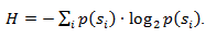
This value is called the entropy of the probability distribution F, or the entropy of the source at a given point in time.
However, usually the probability of the appearance of an element cannot be independent; on the contrary, it depends on some factors. In this case, for each newly encoded element s i, the probability distribution F takes some value F k , that is, for each element F = F k and H = H k .
In other words, it can be said that the source is in the state k, which corresponds to a certain set of probabilities p k (s i ) for all elements s i .
Therefore, given this amendment, it is possible to express the average length of codes as
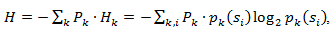
Where P k - the probability of finding the source in the state k.
So, at this stage, we know that compression is based on the replacement of frequently encountered elements with short codes, and vice versa, and also know how to determine the average length of codes. But what is code, coding, and how does it occur?
Memoryless codes are the simplest codes on the basis of which data can be compressed. In a code without memory, each character in the encoded data vector is replaced by a codeword from a prefix set of binary sequences or words.
In my opinion, not the most understandable definition. Consider this topic in more detail.
Let some alphabet be given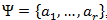 consisting of some (finite) number of letters. Let's call each finite sequence of characters from this alphabet (A = a 1 , a 2 , ..., a n ) a word , and the number n - the length of this word.
Let another alphabet be also given. . Similarly, we denote a word in this alphabet as B.
We introduce two more notation for the set of all non-empty words in the alphabet. Let be - the number of non-empty words in the first alphabet, and
  - in the second.
Suppose also that a mapping F is given, which assigns to each word A from the first alphabet some word B = F (A) from the second. Then the word B will be called the code of the word A, and the transition from the source word to its code will be called coding .
Since a word can also consist of one letter, we can identify the correspondence of the letters of the first alphabet and the corresponding words from the second:
a 1 <-> B 1
a 2 <-> B 2
...
a n <-> B n
This correspondence is called a schema , and is denoted by ∑.
In this case, the words B 1 , B 2 , ..., B n are called elementary codes , and the type of coding with their help is alphabetic coding . Of course, most of us have come across this kind of coding, even if not knowing all the things I described above.
So, we have defined the concepts of alphabet, word, code, and coding . Now we introduce the concept of prefix .
Let the word B have the form B = B'B ''. Then B 'is called the beginning, or prefix of the word B, and B' 'is called its end. This is a fairly simple definition, but it should be noted that for any word B, and some empty word ʌ (“space”), and the word B itself, can be considered both beginnings and ends.
So, we come close to understanding the definition of codes without memory. The last definition that remains for us to understand is the prefix set. The scheme ∑ has the prefix property if for any 1≤i, j≤r, i ≠ j, the word B i is not a prefix of the word B j .
Simply put, a prefix set is a finite set in which no element is the prefix (or beginning) of any other element. A simple example of such a set is, for example, the usual alphabet.
So, we figured out the basic definitions. So how does memoryless encoding happen?
It occurs in three stages.
One of the canonical algorithms that illustrate this method is the Huffman algorithm.
The Huffman algorithm uses the frequency of the appearance of identical bytes in the input data block, and sets in correspondence to frequently occurring blocks of a string of bits of shorter length, and vice versa. This code is the minimum redundant code. Consider the case when, regardless of the input stream, the alphabet of the output stream consists of only 2 characters - zero and one.
First of all, when coding with a Huffman algorithm, we need to construct a scheme ∑. This is done as follows:
Steps 2 and 3 are repeated until only 1 pseudo-character is left in the alphabet, containing all the initial symbols of the alphabet. Moreover, since at each step and for each character, the corresponding word B i changes (by adding one or zero), after this procedure is completed, each initial character of the alphabet a i will correspond to a certain code B i .
For the best illustration, consider a small example.
Suppose we have an alphabet consisting of only four characters - {a 1 , a 2 , a 3 , a 4 }. Suppose also that the probabilities of occurrence of these symbols are equal respectively to p 1 = 0.5; p 2 = 0.24; p 3 = 0.15; p 4 = 0.11 (the sum of all probabilities is obviously equal to one).
So, we will construct the scheme for the given alphabet.
If you make an illustration of this process, you get something like the following:
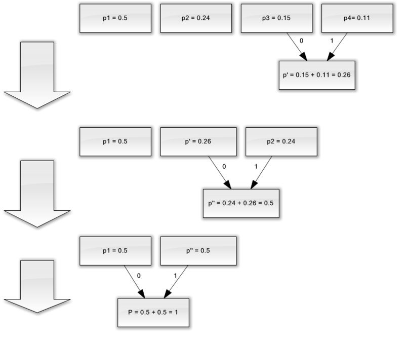
As you can see, with each union we assign codes 0 and 1 to the characters to be joined.
That way, when a tree is built, we can easily get the code for each character. In our case, the codes will look like this:
a 1 = 0
a 2 = 11
a 3 = 100
a 4 = 101
Since none of these codes is a prefix of any other (that is, we have received the notorious prefix set), we can uniquely identify each code in the output stream.
So, we have achieved that the most frequent symbol is encoded by the shortest code, and vice versa.
If we assume that initially one byte was used to store each character, then we can calculate how much we managed to reduce the data.
Suppose that at the input we had a line of 1000 characters in which the character a 1 was encountered 500 times, a 2 - 240, a 3 - 150, and a 4 - 110 times.
Initially, this line occupied 8000 bits. After coding, we get a string long in ∑p i l i = 500 * 1 + 240 * 2 + 150 * 3 + 110 * 3 = 1760 bits. So, we managed to compress the data 4.54 times, spending an average of 1.76 bits on encoding each character of the stream.
Let me remind you that according to Shannon, the average code length is . Substituting our probabilities into this equation, we obtain an average code length of 1.75496602732291, which is very, very close to the result we obtained.
However, it should be borne in mind that in addition to the data itself, we need to store the coding table, which will slightly increase the total size of the encoded data. It is obvious that in different cases different variations of the algorithm can be used - for example, sometimes it is more efficient to use a predetermined probability table, and sometimes it is necessary to compile it dynamically by traversing compressible data.
So, in this article I tried to talk about the general principles by which lossless compression occurs, and also considered one of the canonical algorithms - Huffman coding.
If the article comes to taste to the habrosocommunity, then I will gladly write a sequel, as there are many more interesting things related to lossless compression; these are both classical algorithms and preliminary data transformations (for example, the Burrows-Wheeler transformation), and, of course, specific algorithms for compressing sound, video and images (the most interesting topic, in my opinion).
Today I want to touch on the topic of lossless data compression. Despite the fact that there were already articles on some algorithms in Habré, I wanted to talk about this in a little more detail.
I will try to give both a mathematical description and a description in the usual way, so that everyone can find something interesting for themselves.
In this article I will touch on the fundamental moments of compression and the main types of algorithms.
Compression. Do we need it in our time?
')
Of course, yes. Of course, we all understand that now we have access to both large-capacity storage media and high-speed data transmission channels. However, at the same time, the volumes of transmitted information are growing. If several years ago we watched 700-megabyte movies that fit on one disc, then today films in HD quality can occupy dozens of gigabytes.
Of course, there is not much benefit from compressing everything. But still there are situations in which compression is extremely useful if not necessary.
- Sending documents by e-mail (especially large volumes of documents using mobile devices)
- When publishing documents on sites, the need to save traffic
- Saving disk space in cases when replacing or adding storage is difficult. For example, this happens in cases where knocking out a budget for capital expenditure is not easy, and there is not enough disk space.
Of course, you can come up with many more different situations in which compression will be useful, but these few examples are enough for us.
All compression methods can be divided into two large groups: lossy compression and lossless compression. Lossless compression is used in cases where the information needs to be restored to within a bit. This approach is the only possible compression, for example, text data.
In some cases, however, exact information recovery is not required and it is allowed to use algorithms that implement lossy compression, which, unlike lossless compression, is usually easier to implement and provides a higher degree of archiving.
| Lossy compression |
| Better compression rates, while maintaining “good enough” data quality. They are mainly used to compress analog data - sound, images. In such cases, the unpacked file may be very different from the original at the bit-to-bit level of comparison, but it is almost indistinguishable to the human ear or eye in most practical applications. |
| Lossless compression |
| The data is restored to within a bit, which does not lead to any loss of information. However, lossless compression usually shows the worst compression ratios. |
So, we proceed to the consideration of lossless compression algorithms.
Universal lossless compression methods
In general, there are three basic options on which compression algorithms are built.
The first group of methods is stream conversion. This involves the description of new incoming uncompressed data through already processed. No probabilities are calculated, the coding of symbols is carried out only on the basis of the data that have already been processed, such as in the LZ methods (named for Abraham Lempel and Jacob Ziv). In this case, the second and further occurrences of a certain substring already known to the encoder are replaced with references to its first occurrence.
The second group of methods is statistical compression methods. In turn, these methods are divided into adaptive (or flow), and block.
In the first (adaptive) version, the calculation of probabilities for new data occurs from data already processed during coding. These methods include adaptive versions of Huffman and Shannon-Fano algorithms.
In the second (block) case, the statistics of each data block is calculated separately, and added to the most compressed block. These include static variants of Huffman, Shannon-Fano, and arithmetic coding.
The third group of methods is the so-called block conversion methods. Incoming data is divided into blocks, which are then transformed as a whole. However, some methods, especially those based on permutation of blocks, may not lead to a significant (or even any) reduction in the amount of data. However, after such processing, the data structure is significantly improved, and the subsequent compression by other algorithms is more successful and fast.
General principles on which data compression is based
All data compression methods are based on a simple logical principle. If we imagine that the most common elements are encoded with shorter codes, and less frequently, longer ones, then all the data will require less space to store than if all the elements were represented by codes of the same length.
The exact relationship between the frequencies of appearance of elements, and the optimal lengths of codes is described in the so-called Shannon's source coding theorem, which defines the limit of maximum lossless compression and Shannon's entropy.
A bit of math
If the probability of occurrence of the element s i is equal to p (s i ), then it will be most advantageous to represent this element - log 2 p (s i ) bits. If during coding it is possible to ensure that the length of all elements will be reduced to log 2 p (s i ) bits, then the length of the entire coding sequence will be minimal for all possible coding methods. Moreover, if the probability distribution of all elements F = {p (s i )} is constant, and the probabilities of the elements are mutually independent, then the average length of the codes can be calculated as
This value is called the entropy of the probability distribution F, or the entropy of the source at a given point in time.
However, usually the probability of the appearance of an element cannot be independent; on the contrary, it depends on some factors. In this case, for each newly encoded element s i, the probability distribution F takes some value F k , that is, for each element F = F k and H = H k .
In other words, it can be said that the source is in the state k, which corresponds to a certain set of probabilities p k (s i ) for all elements s i .
Therefore, given this amendment, it is possible to express the average length of codes as
Where P k - the probability of finding the source in the state k.
So, at this stage, we know that compression is based on the replacement of frequently encountered elements with short codes, and vice versa, and also know how to determine the average length of codes. But what is code, coding, and how does it occur?
Memory coding
Memoryless codes are the simplest codes on the basis of which data can be compressed. In a code without memory, each character in the encoded data vector is replaced by a codeword from a prefix set of binary sequences or words.
In my opinion, not the most understandable definition. Consider this topic in more detail.
Let some alphabet be given
consisting of some (finite) number of letters. Let's call each finite sequence of characters from this alphabet (A = a 1 , a 2 , ..., a n ) a word , and the number n - the length of this word.Let another alphabet be also given.
. Similarly, we denote a word in this alphabet as B.We introduce two more notation for the set of all non-empty words in the alphabet. Let be
- the number of non-empty words in the first alphabet, and - in the second.Suppose also that a mapping F is given, which assigns to each word A from the first alphabet some word B = F (A) from the second. Then the word B will be called the code of the word A, and the transition from the source word to its code will be called coding .
Since a word can also consist of one letter, we can identify the correspondence of the letters of the first alphabet and the corresponding words from the second:
a 1 <-> B 1
a 2 <-> B 2
...
a n <-> B n
This correspondence is called a schema , and is denoted by ∑.
In this case, the words B 1 , B 2 , ..., B n are called elementary codes , and the type of coding with their help is alphabetic coding . Of course, most of us have come across this kind of coding, even if not knowing all the things I described above.
So, we have defined the concepts of alphabet, word, code, and coding . Now we introduce the concept of prefix .
Let the word B have the form B = B'B ''. Then B 'is called the beginning, or prefix of the word B, and B' 'is called its end. This is a fairly simple definition, but it should be noted that for any word B, and some empty word ʌ (“space”), and the word B itself, can be considered both beginnings and ends.
So, we come close to understanding the definition of codes without memory. The last definition that remains for us to understand is the prefix set. The scheme ∑ has the prefix property if for any 1≤i, j≤r, i ≠ j, the word B i is not a prefix of the word B j .
Simply put, a prefix set is a finite set in which no element is the prefix (or beginning) of any other element. A simple example of such a set is, for example, the usual alphabet.
So, we figured out the basic definitions. So how does memoryless encoding happen?
It occurs in three stages.
- An alphabet Ψ of the symbols of the original message is composed, and the symbols of the alphabet are sorted in descending order of probability in the message.
- Each character a i from the alphabet Ψ is associated with a certain word B i from the prefix set Ω.
- Each character is encoded, followed by combining the codes into one data stream, which will be the results of compression.
One of the canonical algorithms that illustrate this method is the Huffman algorithm.
Huffman Algorithm
The Huffman algorithm uses the frequency of the appearance of identical bytes in the input data block, and sets in correspondence to frequently occurring blocks of a string of bits of shorter length, and vice versa. This code is the minimum redundant code. Consider the case when, regardless of the input stream, the alphabet of the output stream consists of only 2 characters - zero and one.
First of all, when coding with a Huffman algorithm, we need to construct a scheme ∑. This is done as follows:
- All letters of the input alphabet are ordered in decreasing order of probability. All words from the output stream alphabet (that is, what we will encode) are initially considered empty (recall that the output stream alphabet consists only of {0,1} characters).
- The two characters a j-1 and a j of the input stream, which have the smallest probabilities of occurrence, are combined into one “pseudo-symbol” with probability p equal to the sum of the probabilities of the characters included in it. Then we append 0 to the beginning of the word B j-1 , and 1 to the beginning of the word B j , which will subsequently be the character codes a j-1 and a j, respectively.
- We delete these characters from the alphabet of the original message, but we add the formed pseudo-character to this alphabet (naturally, it should be inserted into the alphabet at the right place, taking into account its probability).
Steps 2 and 3 are repeated until only 1 pseudo-character is left in the alphabet, containing all the initial symbols of the alphabet. Moreover, since at each step and for each character, the corresponding word B i changes (by adding one or zero), after this procedure is completed, each initial character of the alphabet a i will correspond to a certain code B i .
For the best illustration, consider a small example.
Suppose we have an alphabet consisting of only four characters - {a 1 , a 2 , a 3 , a 4 }. Suppose also that the probabilities of occurrence of these symbols are equal respectively to p 1 = 0.5; p 2 = 0.24; p 3 = 0.15; p 4 = 0.11 (the sum of all probabilities is obviously equal to one).
So, we will construct the scheme for the given alphabet.
- We combine the two characters with the smallest probabilities (0.11 and 0.15) into the pseudo-character p '.
- Remove the combined characters, and insert the resulting pseudo-character into the alphabet.
- We combine the two characters with the smallest probability (0.24 and 0.26) into the pseudo-character p ''.
- Remove the combined characters, and insert the resulting pseudo-character into the alphabet.
- Finally, combine the remaining two characters, and get the top of the tree.
If you make an illustration of this process, you get something like the following:
As you can see, with each union we assign codes 0 and 1 to the characters to be joined.
That way, when a tree is built, we can easily get the code for each character. In our case, the codes will look like this:
a 1 = 0
a 2 = 11
a 3 = 100
a 4 = 101
Since none of these codes is a prefix of any other (that is, we have received the notorious prefix set), we can uniquely identify each code in the output stream.
So, we have achieved that the most frequent symbol is encoded by the shortest code, and vice versa.
If we assume that initially one byte was used to store each character, then we can calculate how much we managed to reduce the data.
Suppose that at the input we had a line of 1000 characters in which the character a 1 was encountered 500 times, a 2 - 240, a 3 - 150, and a 4 - 110 times.
Initially, this line occupied 8000 bits. After coding, we get a string long in ∑p i l i = 500 * 1 + 240 * 2 + 150 * 3 + 110 * 3 = 1760 bits. So, we managed to compress the data 4.54 times, spending an average of 1.76 bits on encoding each character of the stream.
Let me remind you that according to Shannon, the average code length is
. Substituting our probabilities into this equation, we obtain an average code length of 1.75496602732291, which is very, very close to the result we obtained.However, it should be borne in mind that in addition to the data itself, we need to store the coding table, which will slightly increase the total size of the encoded data. It is obvious that in different cases different variations of the algorithm can be used - for example, sometimes it is more efficient to use a predetermined probability table, and sometimes it is necessary to compile it dynamically by traversing compressible data.
Conclusion
So, in this article I tried to talk about the general principles by which lossless compression occurs, and also considered one of the canonical algorithms - Huffman coding.
If the article comes to taste to the habrosocommunity, then I will gladly write a sequel, as there are many more interesting things related to lossless compression; these are both classical algorithms and preliminary data transformations (for example, the Burrows-Wheeler transformation), and, of course, specific algorithms for compressing sound, video and images (the most interesting topic, in my opinion).
Literature
- Vatolin D., Ratushnyak A., Smirnov M. Yukin V. Data Compression Methods. Device archivers, image and video compression; ISBN 5-86404-170-X; 2003
- D. Salomon. Compression of data, image and sound; ISBN 5-94836-027-X; 2004
- www.wikipedia.org
Source: https://habr.com/ru/post/142242/
All Articles