Recommended systems: SVD on perl
In the previous series, we discussed what a singular value decomposition (SVD) is and formulated a singular value model with basic predictors. Last time, we have already brought the matter to specific update formulas. Today I will demonstrate a very simple implementation of a very simple model, we will apply it to the already familiar rating matrix, and then we will discuss what the results are.

So, SVD on Perl. Ready script that can be run as
As you can see, absolutely nothing terrible - you just need to start the process of updating the scales and continue it until convergence. The convergence is determined by the RMSE (root mean squared error) - root-mean-square error, i.e. the root of the sum of squares of errors divided by the number of test cases. We implement a stochastic gradient descent: after each test case, we immediately change the parameters, and do not collect error statistics for the entire database.
')
When RMSE ceases to improve noticeably, we decrease the speed of learning; With this approach, sooner or later the process should converge (ie, the RMSE should stop changing). What is λ here, we will discuss next time, today it will be zero in our examples.
Now let's apply what we did to the rating matrix, which we considered in one of the first texts .
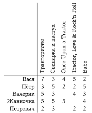
In a suitable format, you can download it here (order is preserved). After running our script on this dataset, we’ll get something like the following.
But the most interesting thing is that we got a reasonable decomposition of the remaining user preferences into two factors. An example, of course, is a toy one, and in dataset it was originally laid down that films are divided into films “about pigs” and “about tractors”; Some users are more fond of powerful technology, and some - pork hryashik.
Indeed, it is clear that the first factor is how much the film is “about tractors”, and the second factor is how much it is “about pigs”; specific values do not have a deep meaning, only their relationship is important.
By the way, I didn’t specifically customized dataset, and in this case there was a funny case with signs: SVD taught negative values of “about tractors” factors for two users who like tractors, Vasya and Valerik. But at the same time, SVD has taught negative values for the “about tractors” factors in films that are really about tractors - a minus to a minus will give a plus. And just 1.0220 Peter, on the contrary, means that he is not at all interested in tractors compared to piglets ...
We can now predict the value of Vasya’s rating for “Tractor drivers” as
Well, it was really possible to assume that Vasya would like Tractorists.
Next time we will talk about overfitting and regularization - what it is, why it is needed and how to implement it in SVD.
So, SVD on Perl. Ready script that can be run as
./svd.pl _ dataset.csv # SVD: , while (abs($old_rmse - $rmse) > 0.00001 ) { $old_rmse = $rmse; $rmse = 0; foreach my $u ( keys %l ) { foreach my $v ( keys %{$l{$u}} ) { # $err = $l{$u}{$v} - ($mu + $b_u[$u] + $b_v[$v] + dot($u_f[$u], $v_f[$v]) ); # $rmse += $err * $err; # ... $mu += $eta * $err; $b_u[$u] += $eta * ($err - $lambda2 * $b_u[$u]); $b_v[$v] += $eta * ($err - $lambda2 * $b_v[$v]); # ... for (my $f=0; $f < $features; ++$f) { $u_f[$u][$f] += $eta * ($err * $v_f[$v][$f] - $lambda2 * $u_f[$u][$f]); $v_f[$v][$f] += $eta * ($err * $u_f[$u][$f] - $lambda2 * $v_f[$v][$f]); } } } ++$iter_no; # , RMSE $rmse = sqrt($rmse / $total); print "Iteration $iter_no:\tRMSE=" . $rmse . "\n"; # RMSE , if ($rmse > $old_rmse - $threshold) { $eta = $eta * 0.66; $threshold = $threshold * 0.5; } } As you can see, absolutely nothing terrible - you just need to start the process of updating the scales and continue it until convergence. The convergence is determined by the RMSE (root mean squared error) - root-mean-square error, i.e. the root of the sum of squares of errors divided by the number of test cases. We implement a stochastic gradient descent: after each test case, we immediately change the parameters, and do not collect error statistics for the entire database.
')
When RMSE ceases to improve noticeably, we decrease the speed of learning; With this approach, sooner or later the process should converge (ie, the RMSE should stop changing). What is λ here, we will discuss next time, today it will be zero in our examples.
Now let's apply what we did to the rating matrix, which we considered in one of the first texts .
In a suitable format, you can download it here (order is preserved). After running our script on this dataset, we’ll get something like the following.
  Read 5 users and 5 urls.
 Iteration 1: RMSE = 1.92845291697284
 Iteration 2: RMSE = 1.28481736445124
 Iteration 3: RMSE = 1.14159530044051
 ...
 Iteration 808: RMSE = 0.0580161117835789
 Iteration 809: RMSE = 0.0580061123741253
        mu: 2.54559533638261
 User base: 0.7271 0.1626 0.7139 1.9097 -0.9677
 Item base: 0.8450 0.6593 0.2731 0.7328 0.0354
 User features
   user 0: -0.5087 -0.8326
   user 1: 1.0220 1.2826
   user 2: -0.9509 0.2792
   user 3: 0.1031 -0.4814
   user 4: 0.6095 0.0557
 Item features:
   Item 0: -0.8368 0.2511
   item 1: 1.1101 0.4120
   item 2: -0.4159 -0.4073
   item 3: -0.3130 -0.9115
item 4: 0.6408 1.2205 But the most interesting thing is that we got a reasonable decomposition of the remaining user preferences into two factors. An example, of course, is a toy one, and in dataset it was originally laid down that films are divided into films “about pigs” and “about tractors”; Some users are more fond of powerful technology, and some - pork hryashik.
Indeed, it is clear that the first factor is how much the film is “about tractors”, and the second factor is how much it is “about pigs”; specific values do not have a deep meaning, only their relationship is important.
By the way, I didn’t specifically customized dataset, and in this case there was a funny case with signs: SVD taught negative values of “about tractors” factors for two users who like tractors, Vasya and Valerik. But at the same time, SVD has taught negative values for the “about tractors” factors in films that are really about tractors - a minus to a minus will give a plus. And just 1.0220 Peter, on the contrary, means that he is not at all interested in tractors compared to piglets ...
We can now predict the value of Vasya’s rating for “Tractor drivers” as
2.5456 + 0.7271 + 0.8450 + (-0.5087) * (- 0.8368) + (-0.8326) * 0.2511 = 4.3343143.
Well, it was really possible to assume that Vasya would like Tractorists.
Next time we will talk about overfitting and regularization - what it is, why it is needed and how to implement it in SVD.
Source: https://habr.com/ru/post/141959/
All Articles