Rendering the other way around. GPU Hough Transformation

Hough Transform is used to search on the image of the figures specified analytically: straight lines, circles and any others, for which you can come up with an equation with a small number of parameters. Much has been written about the conversion of Khaf, and this article does not set a goal to highlight in detail all aspects. I will only explain the general principle, focusing on the features that prevent its implementation on the GPU "head on" and, of course, I will offer a solution. Those who know the problems and want to see a solution immediately can skip a couple of sections.

Algorithm for CPU

First, we describe the desired shape by an equation. For example, for a line, this could be y = Ax + B.
Then we start the so-called accumulator: an array with the number of measurements equal to the number of parameters in the equation. In our case - two-dimensional. We will have the Space of Hough (at least part of it) - in it the straight lines will be represented by their parameters. For example, A is horizontal and B is vertical. One line in ordinary space = one point in Hough space.
')
The original image is binarized, and for each non-empty point (x ₀ , y ₀ ) we define a set of lines that can pass through this point: y ₀ = Ax ₀ + B. Here x ₀ and y ₀ are constant, A and B are variables, and This equation defines a straight line in Hough space. We need to draw this line in our battery - add 1 to each element through which it passes. Such a procedure is called voting: a dot votes for the direct ones that can pass through it.

As a result, it turns out that all the votes from all points are collected in the accumulator, and it can be considered that the “winners of the vote” are present on the original image. Here, of course, it is possible and necessary to apply threshold filtering and other methods in order to find maxima in the Hough space, but the main and most laborious task is to fill the battery.

Wikipedia illustration:

GPU issues

A GPU can be considered as a set (up to thousands) of small processors having a common memory, and, as a rule, the algorithms are simply divided: giving each processor its own piece of work. It would seem that we divide the original image into pieces, give each processor its own piece - and that's it. But no, we cannot divide the battery: in each piece of the original image there can be points projected onto any place of the Hough space. Processors cannot write to the general memory, only to read - otherwise there will be problems with synchronization. The solution would be to give each processor its own battery, and after processing, add up the batteries together. But, you remember, thousands of processors. Even if there is so much memory, the time for its allocation and processing will override the benefits of parallel execution of the algorithm.

Another, smaller, problem is the algorithms for “drawing” lines in the Hough space. They can be quite intricate, but even the simplest ones will contain loops and branching. But the GPU does not like this: small processors do not know how to execute each of their programs, they all perform one (well, not all, but in large groups). Simply everyone operates with the data. This means that both branches of the branch are executed (then the result of the unnecessary is discarded for each processor separately). And the loop is executed as many times as necessary for the worst case input. This leads to the fact that the efficiency of the use of processors decreases.

Algorithm modification for GPU

My initial idea was this: why not divide into “zones of influence” not the original image, but the Hough space? That is, let's calculate the value for each point of the Hough space separately. At first glance, this seems silly: any point of the original image can give a “voice”, which means that we will have to examine them all. Total number of read operations = [number of points of the original image] x [number of battery cells] , whereas in the traditional way it is only [number of points of the original image] .

But then the number of write operations is potentially reduced — [the number of battery cells] versus [the number of non-empty points] x [the average length of the image of a point in Hough space] . If there are a lot of non-empty points, the difference is significant.

So the reading gets bigger, the writing gets smaller, and it becomes more orderly. Now we remember what the power of the GPU is. In reading speed! Video cards are equipped with fast memory, access to it is “straightened” to the limit - all with the aim to impose textures as quickly as possible. True, this is at the expense of latency - unordered read requests are slower. But we will not have these.

The second idea. If it is necessary to “draw” in the space of Hafa - why not use the “drawing” talents of video cards? Let's overlay the original image on the Hough space as a texture.

This leads to the fact that in my method neither the OpenCL or CUDA code, nor the shaders are needed. The video card is not even obliged to support them in order to get an image of the Hough space. The price for this is non-universality: in practice, these are two essentially different methods: one for circles and the other for straight lines. It seems that the “circles” method can be applied to any closed lines and any figures with three or more parameters in the equation, but the efficiency may be different.

The method of "circles"

The circle is described by an equation with three parameters - (xx ₀ ) ² + (yy ₀ ) ² = R ² . Here (x ₀ , y ₀ ) are the coordinates of the center, and R is the radius. The Hough space should have three dimensions, but for now we restrict ourselves to two and fix R (let's say we know it). In this case, all we need to find is the coordinates of the center (s).

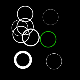
Take this original image (all circles of one radius)


and, having made it almost transparent, we impose on ourselves as follows:


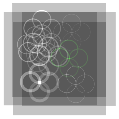
All images are offset from the original by the radius of the circle. The angle between adjacent offset radii is the same. That is, for example, the upper left corners of the images are distributed around a circle of the same radius as the desired one.

For clarity of illustration, I put the inverse of the original image below and marked the important places in red.


Each circle of each image passes through the center of the corresponding circle of the original image. At these points they overlap each other and the maximum brightness is obtained.

This is what will happen if you do this operation 32 times:


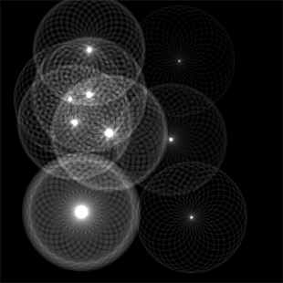
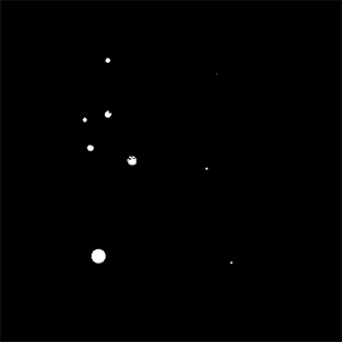
And after the threshold filtering:


Thus, we have filled two dimensions of Hough space. Now, by varying the radius, you can easily fill the third. And you can not try to accumulate all 3 measurements in memory, and process the resulting image, keeping the position of the centers and the radius and free the memory.

The code (Managed DirectX, the full version is the link below), creating well-spaced rectangles:

float r = (float)rAbs / targetSize; for (int i = 0; i < n; i++) { double angle = 2 * Math.PI / n * i; rectangles.Add(new TexturedRect(new Vector2(1f, 1f), new Vector2((float)(Math.Cos(angle) * r), (float)(Math.Sin(angle) * r)), new Vector2(1f, 1f), new Vector2(0f, 0f), 0)); } 

Code setting alpha transparency in the right way:

 device.RenderState.AlphaBlendEnable = true, device.RenderState.BlendFactor = (byte)(256.0 * brightness / n) device.RenderState.BlendOperation = BlendOperation.Add; device.RenderState.SourceBlend = Blend.BlendFactor; device.RenderState.DestinationBlend = Blend.One; 

Here rAbs sets the desired radius, brightness - brightness, n - the number of layers.

Render everything in texture

 new Microsoft.DirectX.Direct3D.Texture(device, targetSize, targetSize, 1, Usage.RenderTarget, cbGray.Checked ? Format.L8 : Format.X8R8G8B8, Pool.Default); dxPanel.RenderToTexture(new Options() { AlphaBlendEnable = true, BlendFactor = (byte)(256.0 * (tbBrightness.Value / 100.0) / n) }, rectangles); 

And you can use a 3D texture and several sets of layers in order to render all the radii of interest and at the same time get the three-dimensional space of Hough (I did not try to do that).

With transparency, there is such a nuance that if you use an 8-bit color and a sufficiently large number of layers, then the BlendFactor will be less than 10, up to 1. This can lead to large rounding errors, and a stepwise change in brightness, if you adjust the overall brightness with BlendFactor. However, if the brightness is not adjusted, it will be difficult to choose a threshold value for filtering all due to the same rounding errors. Also, if you use an image with shades of gray, the shades will suffer, and even I will be lost with BlendFactor = 1.

This problem can be solved by using a large color depth for the render target (for example, 16 or 32 bits), if the video card supports it.

Here is another example of working on a noisy image. Original:


Result (64 layers):



You may notice that the algorithm most likely polls not all the points that make up the circle (unless the circle is too small). With the increase in the number of layers, the percentage of surveyed points and the accuracy of determination increases, but the operation time increases and the problems described above appear.

The method of "direct"

Anisotropic filtering

Before proceeding to the description of the method itself, you need to make a digression and tell more about anisotropic filtering in video cards. When overlaying a texture, it can happen that the color of a single screen pixel should define several texture points (texels). This usually happens either with a large distance of the polygon from the viewer, or with a strong inclination of the polygon (a good example is the texture of the road). And if in the first case it is possible to scale the texture into several resolutions in advance, and then take the necessary variant (mip-mapping), then in the second one cannot do it because the texture can be turned “towards the viewer” either side.


And here the video cards use all sorts of tricks, but the most honest way is to take all the texels from the projection of the pixel on the texture and calculate their average value. This is called anisotropic (direction dependent) filtering.

The maximum traditionally supported level of anisotropic filtering is 16 (apparently texels).

About the method itself

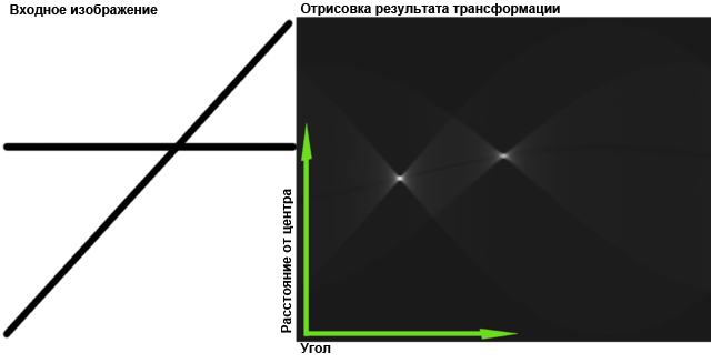
Take our image and "flatten" it, for example, vertically. Those. render it entirely on a 1-pixel-high rectangle. Ideally, the vertical lines will turn into points (maxima). Everything else will be smeared. Thus, we have already obtained the value of one parameter — this is the distance from the left edge of the image to the point (to the line on the original image).

Now take a fresh copy of the image, but before flattening it, turn it to some small angle around the center of the image in a clockwise direction. Then flatten. Some lines will go to points. These will be the straight lines that are inclined at the same angle of rotation of the image.

Thus, going through all the angles from 0 to Pi, we get the values ​​of the second parameter - the angle of rotation of the picture. By these two parameters, you can restore any original line.

The only question that remains is how to properly flatten the image. If you do it in the forehead, only noise will remain - anisotropic filtering will work, but it will take only 16 texels (pixels of the original image). This is most likely too little.

You can cut the image into rectangles 16 pixels wide, flatten each one separately,


and then draw them on top of each other, as we did in the method with circles. This will work, and as a result, each pixel will be taken into account.


(We can assume that the pictures are enlarged 4 times so that the details can be seen)

If the image is higher than 16 * 256 = 4096 pixels, you can cut it into rectangles of greater height, or use a greater color depth. But, most likely, such an image simply does not fit into the texture.

In order not to lose the lines in the corners, or near the short sides of the non-square image, you must take the render target width equal to the diagonal of the original image.

The code that sets up the texture sampler (I rotate the texture coordinates, so I need the sampler to return black if there is no texture somewhere because of the rotation).

 device.SamplerState[0].MinFilter = TextureFilter.Anisotropic; device.SamplerState[0].MaxAnisotropy = 16; device.SamplerState[0].AddressU = TextureAddress.Border; device.SamplerState[0].AddressV = TextureAddress.Border; device.SamplerState[0].AddressW = TextureAddress.Border; device.SamplerState[0].BorderColor = Color.Black; 

Creating Rectangles

 double sourceRectPixelWidth = sourceSize / n; double targetRectPixelWidth = Math.Ceiling(sourceRectPixelWidth / anizotropy); int angleValues = (int)Math.Floor(targetSize / targetRectPixelWidth); float sourceRectWidth = (float)(sourceRectPixelWidth / sourceSize); float tarectRectWidth = (float)(targetRectPixelWidth / targetSize); for (int angleNumber = 0; angleNumber < angleValues; angleNumber++) { double angle = Math.PI / angleValues * angleNumber; float targetShift = tarectRectWidth * angleNumber; for (int sliceNumber = 0; sliceNumber < n; sliceNumber++) { float sourceShift = sourceRectWidth * sliceNumber; rectangles.Add(new TexturedRect( new Vector2(tarectRectWidth, 1f), new Vector2(targetShift, 0f), new Vector2(sourceRectWidth, 1f), new Vector2(sourceShift, 0f), (float)angle)); } } 

The same noisy image as in the last section, but now we are looking for lines (32 layers, 512 steps of the angle of rotation):

Extension of the "circles" method

Images can be shifted not along the radii of circles, but in a more capricious way. For example, choose some arbitrary desired contour (not even expressed using a formula) and a certain point O.



Then, successively choosing points A1, A2 on the contour, shift the image layers by vectors AO. It turns out that the angle of the images describes a figure like this.



In this case, all the bears in the image will be found - the maxima will fall on the point corresponding to the point O of the original contour.

Additional advantages over the traditional way

• Saving memory (you can not save all measurements in memory)
  
• You can not do binarization, and use shades of gray. This will not affect performance and may increase accuracy.
  
• You can evenly ignore part of the points in favor of speed (In the traditional way, you can also do this, but you have to resort to all sorts of tricks to achieve uniformity, and not just skip some angle)
  
• You can work with very noisy images, it will not reduce the speed
  
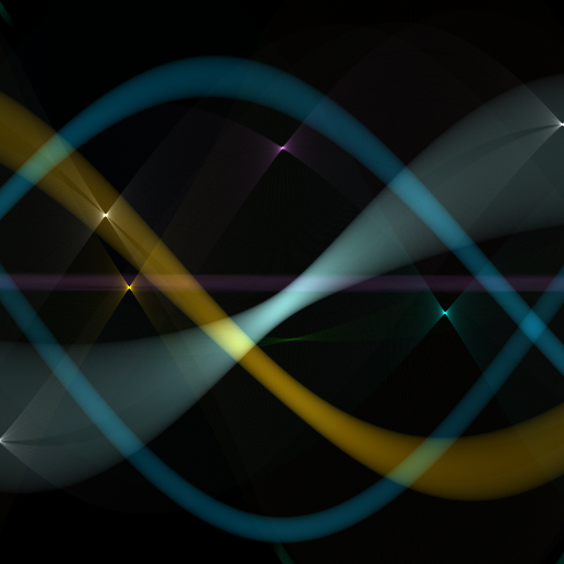
• Bonus You can use color images to get beautiful pictures like the one on KPDV
  

Performance

It will not be very fair to compare the performance of a pure counting between a CPU and a GPU, since one of the hardest parts of working with a GPU is loading and unloading data. It is hardly worth uploading the results of the raw work back to the CPU. You can try compacting them first to upload only the found shape parameters, not the points. However, data compaction is also quite cunningly implemented on the GPU, so I haven’t even taken it for now.

Pure conversion performance hafa. Input and output - 2048 * 2048, GPU - GeForce GTS250:


For comparison, the results of the detection of lines using OpenCV. The input is 2048 * 2048, the output is 2048 distance steps between the lines, CPU is Core i5 750 @ 3700Mhz.


From this time, 50-80 ms goes to the Canny border detector (after which a two-color image is processed).

Conclusion: in the detection of lines on images with a small number of GPU details, it is 5–20 times faster. On noisy / detailed images, the speed increase can be 100 to 300 times.

It was not possible to compare the speed of detecting circles, since OpenCV uses not the usual, but the gradient Hough method .

Materials on the topic

Project sources (To build you need DirectX SDK June 2010)
Hough Transformation
Hough's algorithm for detecting arbitrary curves in images
Hough Transform on GPU
Gradient Hough Method in OpenCV

UPD: Yes, in order to run the attached example you need .NET and DirectX, but the principle itself is not tied to them. With the same success, you can implement it in c ++ and OpenGL. CUDA and OpenCL are still not needed.