OpenMP Optimization
The gradual development of the project went on as usual.
For a part of the funds received under the grant, the personal computer equipment park was updated. As a result, the calculations are now carried out not on a long-suffering laptop, but on a perfectly acceptable machine with a pseudo-eight-core Intel Core i7-2600 and 8 Gb of RAM on board. And the development is done under Visual Studio 2005 (obtained through the DreamSpark program) with the connected trial version of the Intel FORTRAN Compiler 12 / Intel Parallel Studio XE 2011 (it all runs under Win 7). OpenMP is used as a parallel API.
In view of the obviously noticeable growth of available capacities, new negative features of the algorithm written earlier were found. First of all, since March, a deep optimization of the computational part of the code was carried out, which made it possible to gain about 70% in performance. Such an increase was ensured primarily by the elimination of division operations, as well as an increase in the number of predictable variables.
')
upd: The post, in general, is about the gray working everyday life, and does not contain any discoveries in itself.
The program was regularly used and produced good results, until one day it was decided to check how well the parallelization was performed. And, rather, even expectedly, than surprisingly, execution in one thread turned out to be on average twice as fast as multi-threaded launches, regardless of the number of threads.
The answer, in general, lies on the surface. From the mathematical point of view, the algorithm was optimized to such an extent that its bottleneck was the exchange of data between individual streams, which was confirmed even by a brief analysis in the Intel Vtune Amplifier. The greatest time required to initialize the threads and their local variables, as well as access to common variables and arrays. A significant role in the visibility of the dirty trick was played by the fact that until now a rough computational grid was used, only 3x200 spatial nodes (a kind of imitation of a one-dimensional problem), and the computation time was relatively small.
What was done for optimization?
First of all, the directives and the separation of variables into classes are corrected. In particular, the main working arrays in which the values that are the purpose of the calculation are stored from
Here lists of variables are omitted, because with them the code takes about a dozen lines.
In total, there are nine such places in the code. Nine bottlenecks through which the program, quoting M. Evdokimov, "Squeaks, but climbs."
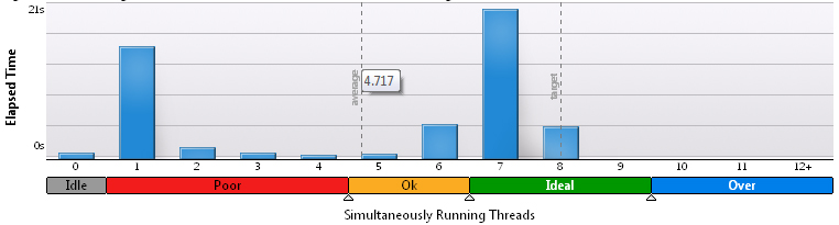
Throwing different variables back and forth lasted a couple of evenings, but the optimality of work could not be considered. The launch on a full processor load showed that on average only 2.1 - 2.3 threads simultaneously exist. Processor time was spent regularly in eight times. For clarity, histograms from VTune Amplifier for 3x200 grid:

For 100x100:
For 200x200:
Obviously, as the share of computations increases, the results improve, but there is no desire to call it such a high efficiency.
Applying forced sleep deprivation to streams by increasing the KMP_BLOCKTIME value from 200 ms to 10 s just a little helped in the same way.
Unexpectedly, a stern look was cast on the "space-time" structure formed by the flows in the algorithm. And everything immediately fell into place. The weak point was the directive
The
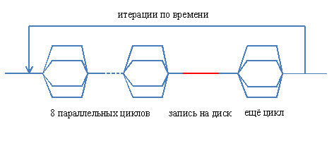
A complete reorganization of the structure of the parallel part of the program was carried out. Now the flow diagram looks like this:

Vertical dashed lines conventionally show the boundaries of parallel loops, and towards the end, the
And in the source text the directive structure looks like this:
That is, the whole cycle body in time (the program makes a direct numerical simulation of the evolution of the hydrodynamic system) is now in a parallel area, the threads are created at the beginning of the iteration and are destroyed only when it is completed, and not resurrected repeatedly. It is no longer possible to wrap in a parallel area and a time cycle, since each iteration of it, of course, is completely dependent on the previous one ( please correct it, if not so - my logic here gives a certain failure ).
The final improvement aimed at speeding up work was disabling the barrier synchronization between the flows in some cycles where it would not affect subsequent calculations.
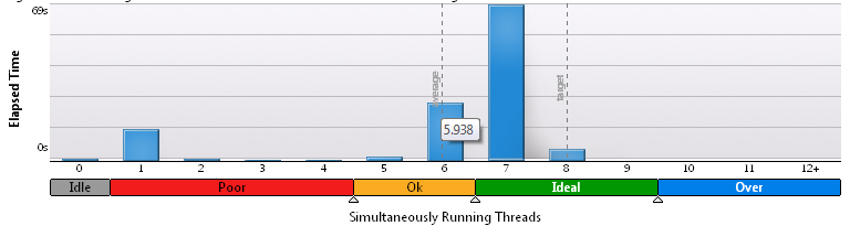
As a result, the time of really parallel code execution seems to be increasing. On the 3x200 grid, the VTune node represents this result:

On the grid 100x100 - this:

Finally, at 200x200 - this:

Thus, we confirm the long-standing truth that on large grids, when there are really many calculations, they take up most of the time and parallelism is effective. On small grids, it is required to optimize the exchange between processes, otherwise the results are not joyful. And despite this, the successive stages occupy a predominant part of the working time.
The question arises, is it worth the work done to optimize the spent time and effort? Check the actual speed of the program. The launch was carried out on the same three different grids with eight streams, and the time to a certain reference point was measured. The control points are different in all cases, therefore, it will be incorrect to compare the absolute values between different grids - 1 million iterations for 3 x 200, 500 thousand for 100 x 100 and 200 thousand for 200 x 200 nodes. The second line in parentheses shows the relative difference in the execution time of the two program options.
It is obvious that the optimization carried out provided a good performance boost.
At the same time, we compare the quality of parallelization, determining in the same way the performance gain with increasing number of threads. Immediately it should be noted that on one stream the calculations may turn out to be faster than on two or three, due to, firstly, the lack of the need to exchange data with neighbors, and secondly, the work of TurboBoost, raising the clock frequency by 400 MHz. Also recall that the physical cores of the processor mentioned at the beginning are only 4, and the acceleration on 8 threads is the result of Hyper-Threading.
Grid 3x200, 1 million iterations:
Grid 100x100, 500 thousand iterations:
If on a small number of nodes the results are ambiguous, to put it mildly, although evidencing in favor of multithreading and optimization success, then on a large number of them - everything is again evident.
Findings? The main conclusion is the same - watch how the flows in the program are born and die. Extending their life may be helpful.
The implemented rearranging of the space-time structure of the streams is described, in particular, here:
Efficient load balancing between threads using OpenMP * . That's just it was read after coming up with a solution. Would save a couple of days, eh.
For a part of the funds received under the grant, the personal computer equipment park was updated. As a result, the calculations are now carried out not on a long-suffering laptop, but on a perfectly acceptable machine with a pseudo-eight-core Intel Core i7-2600 and 8 Gb of RAM on board. And the development is done under Visual Studio 2005 (obtained through the DreamSpark program) with the connected trial version of the Intel FORTRAN Compiler 12 / Intel Parallel Studio XE 2011 (it all runs under Win 7). OpenMP is used as a parallel API.
In view of the obviously noticeable growth of available capacities, new negative features of the algorithm written earlier were found. First of all, since March, a deep optimization of the computational part of the code was carried out, which made it possible to gain about 70% in performance. Such an increase was ensured primarily by the elimination of division operations, as well as an increase in the number of predictable variables.
')
upd: The post, in general, is about the gray working everyday life, and does not contain any discoveries in itself.
Minor mischief
The program was regularly used and produced good results, until one day it was decided to check how well the parallelization was performed. And, rather, even expectedly, than surprisingly, execution in one thread turned out to be on average twice as fast as multi-threaded launches, regardless of the number of threads.
The answer, in general, lies on the surface. From the mathematical point of view, the algorithm was optimized to such an extent that its bottleneck was the exchange of data between individual streams, which was confirmed even by a brief analysis in the Intel Vtune Amplifier. The greatest time required to initialize the threads and their local variables, as well as access to common variables and arrays. A significant role in the visibility of the dirty trick was played by the fact that until now a rough computational grid was used, only 3x200 spatial nodes (a kind of imitation of a one-dimensional problem), and the computation time was relatively small.
Minor fixes
What was done for optimization?
First of all, the directives and the separation of variables into classes are corrected. In particular, the main working arrays in which the values that are the purpose of the calculation are stored from
SHARED were turned into THREADPRIVATE by setting the COMMON attribute (which simultaneously optimized their placement in memory) and COPYIN directives. The precomputed variables were left as SHARED , since the application of FIRSTPRIVATE or COPYIN to them not only did not give a noticeable effect, but also worsened the results. In total, the directive before the main work cycles took something like this: !$OMP PARALLEL DO NUM_THREADS(Threads_number) SCHEDULE(DYNAMIC) & !$OMP PRIVATE(...) & !$OMP COPYIN(...) & !$OMP DEFAULT(SHARED) Here lists of variables are omitted, because with them the code takes about a dozen lines.
In total, there are nine such places in the code. Nine bottlenecks through which the program, quoting M. Evdokimov, "Squeaks, but climbs."
Throwing different variables back and forth lasted a couple of evenings, but the optimality of work could not be considered. The launch on a full processor load showed that on average only 2.1 - 2.3 threads simultaneously exist. Processor time was spent regularly in eight times. For clarity, histograms from VTune Amplifier for 3x200 grid:
For 100x100:
For 200x200:
Obviously, as the share of computations increases, the results improve, but there is no desire to call it such a high efficiency.
Applying forced sleep deprivation to streams by increasing the KMP_BLOCKTIME value from 200 ms to 10 s just a little helped in the same way.
Nonsense is rarely small
Unexpectedly, a stern look was cast on the "space-time" structure formed by the flows in the algorithm. And everything immediately fell into place. The weak point was the directive
!$OMP PARALLEL DO NUM_THREADS(Threads_number) SCHEDULE(DYNAMIC) The
PARALLEL keyword is responsible, as is well known, beyond the boundaries of the parallel and sequential code area. Upon its achievement, the creation of new threads, the redistribution of local variables in their memory and other procedures that require a considerable amount of time occur. There were nine such places, as already mentioned. Accordingly, nine times the streams were created and destroyed, and at the same time between them in some places there were not even consecutive sections. Schematically, it can be represented on this picture:A complete reorganization of the structure of the parallel part of the program was carried out. Now the flow diagram looks like this:
Vertical dashed lines conventionally show the boundaries of parallel loops, and towards the end, the
SINGLE directive is used — it writes the calculation results to a disk, for which the work of all streams, except for one, is suspended. It is at least difficult to parallelize it, although there is an idea to record in one stream and perform a further loop in the others, since He does not depend on writing to disk, or rearrange them in places. But these are details that have nothing to do with the case.And in the source text the directive structure looks like this:
Time_cycle: do n = 0, Nt, 1 !$OMP PARALLEL NUM_THREADS(Threads_number) & !$OMP PRIVATE(...) & !$OMP COPYIN(...) & !$OMP DEFAULT(SHARED) !$OMP DO SCHEDULE(DYNAMIC) ... !$OMP END DO ... 7 !$OMP SINGLE ... !$OMP END SINGLE !$OMP DO SCHEDULE(DYNAMIC) ... !$OMP END DO !$OMP END PARALLEL enddo Tyme_Cycle That is, the whole cycle body in time (the program makes a direct numerical simulation of the evolution of the hydrodynamic system) is now in a parallel area, the threads are created at the beginning of the iteration and are destroyed only when it is completed, and not resurrected repeatedly. It is no longer possible to wrap in a parallel area and a time cycle, since each iteration of it, of course, is completely dependent on the previous one ( please correct it, if not so - my logic here gives a certain failure ).
The final improvement aimed at speeding up work was disabling the barrier synchronization between the flows in some cycles where it would not affect subsequent calculations.
As a result, the time of really parallel code execution seems to be increasing. On the 3x200 grid, the VTune node represents this result:
On the grid 100x100 - this:
Finally, at 200x200 - this:
Thus, we confirm the long-standing truth that on large grids, when there are really many calculations, they take up most of the time and parallelism is effective. On small grids, it is required to optimize the exchange between processes, otherwise the results are not joyful. And despite this, the successive stages occupy a predominant part of the working time.
The question arises, is it worth the work done to optimize the spent time and effort? Check the actual speed of the program. The launch was carried out on the same three different grids with eight streams, and the time to a certain reference point was measured. The control points are different in all cases, therefore, it will be incorrect to compare the absolute values between different grids - 1 million iterations for 3 x 200, 500 thousand for 100 x 100 and 200 thousand for 200 x 200 nodes. The second line in parentheses shows the relative difference in the execution time of the two program options.
| Mesh size | Lead time with |
|---|---|
| 3 x 200, before optimization | 94.4 |
| 3 x 200 optimized | 70.0 (-26%) |
| 100 x 100, before optimization | 352 |
| 100 x 100, optimized | 285 (-19%) |
| 200 x 200, before optimization | 543 |
| 200 x 200 optimized | 436 (-19%) |
It is obvious that the optimization carried out provided a good performance boost.
At the same time, we compare the quality of parallelization, determining in the same way the performance gain with increasing number of threads. Immediately it should be noted that on one stream the calculations may turn out to be faster than on two or three, due to, firstly, the lack of the need to exchange data with neighbors, and secondly, the work of TurboBoost, raising the clock frequency by 400 MHz. Also recall that the physical cores of the processor mentioned at the beginning are only 4, and the acceleration on 8 threads is the result of Hyper-Threading.
Grid 3x200, 1 million iterations:
| The number of threads before optimization | Lead time with |
|---|---|
| one | 80.9 |
| 2 | 88.7 |
| 3 | 84.4 |
| four | 83.7 |
| eight | 94.4 |
| The number of threads after optimization | Lead time with |
| one | 87.9 |
| 2 | 145 |
| 3 | 113 |
| four | 97.8 |
| eight | 70.0 |
Grid 100x100, 500 thousand iterations:
| The number of threads before optimization | Lead time with |
|---|---|
| one | 918 |
| 2 | 736 |
| 3 | 536 |
| four | 431 |
| eight | 352 |
| The number of threads after optimization | Lead time with |
| one | 845 |
| 2 | 528 |
| 3 | 434 |
| four | 381 |
| eight | 285 |
If on a small number of nodes the results are ambiguous, to put it mildly, although evidencing in favor of multithreading and optimization success, then on a large number of them - everything is again evident.
Findings? The main conclusion is the same - watch how the flows in the program are born and die. Extending their life may be helpful.
The implemented rearranging of the space-time structure of the streams is described, in particular, here:
Efficient load balancing between threads using OpenMP * . That's just it was read after coming up with a solution. Would save a couple of days, eh.
Source: https://habr.com/ru/post/141172/
All Articles