Radix Tree structure for data compression

This topic is about the use of Radix Tree on a practical example. A radix tree or a residual tree is a data structure formed on the principle of storing values ​​in a leaf node. Intermediate nodes are an element of the final value. This can be a bit for numbers, a character for strings, or a digit for a number, as in the example below. The above compression algorithm using Radix Tree is used in a real embeded system for storing the parameters of a telephone firewall.

Technical task

So the original data.
Suppose we have a phone book, or more simply, a list of contacts. With every contact
related attribute set. For the program "telephone firewall" - these may be Boolean attributes:
outgoing / incoming call, work during business / non-working time, allow / block or auto answer
when calling. The task is to store a list of contacts and their attributes in the phone’s memory, in a compressed form. In conditions of a limited amount of available memory.

So, a more detailed technical task looks like this:
- There is a .INI file with a set of rules for each number. The rule contains a phone number
and the actual boolean attributes applicable to it. The rooms are unique .
Example .INI file, where 12345 is a phone number:
[RULES]
R0000 = 12345,0,0,0,0,0,0,0,0,0,0,0,0
R0001 = 123764465,0,0,0,0,1,0,1,0,0,0
...
R0765 = ...
')
- Internal rule representation:

class NumberEntry
{
string number ;
bool attCalledNumber ;
bool attCallingNumber ;
bool attInboundCall ;
bool attOutboundCall ;
bool attWorkingHours ;
bool attNonWorkingHours ;
bool attBlocked ;
bool attAllowed ;
bool attPrefix ;
bool attAutoAnswer ;
};

* This source code was highlighted with Source Code Highlighter .

- For the existing set of rules, you should build an intermediate extended graph.
In the Graph, each node can be marked as a sheet. For example, take the following set of hypopthetic numbers:
012345
012346
01234567 #
54647
5463
54638

An intermediate graph should be constructed:

Figure 1. Extended (not compressed) graph from TK.

- Advanced Graph is built according to the following rules:
The last digit of each number in the list indicates a leaf node. Attributes associated with the number only refer to the leaf node. In the graph, any node can be marked as a sheet. For the example above, the number 5 in number 01234 5 represents a leaf node, although it is also part of the number 01234 5 67 #

- After all the numbers are added to the intermediate graph (Expanded), it should be compressed. So that each node of the intermediate graph
(eg 0xxx5xxx #), replaced by a sequence of compact nodes (Compact Nodes, without 'x').

The nodes of the extended and compact graph are represented by the following structures:

#pragma pack(push, 1) // 1 MS C++
#define K_MAX_EXPANDED_NODES 12 // . 0-9, * #
struct SG_Y_DigitElement // , 4
{
UINT digit : 4; // 0-9 . '*' 0xA, '#' 0xB. 12 , 4
UINT nextNodeOffset : 13; // ,
BOOL leafNode : 1; // ?

BOOL attCalledNumber : 1; // .
BOOL attCallingNumber : 1;
BOOL attInboundCall : 1;
BOOL attOutboundCall : 1;
BOOL attWorkingHours : 1;
BOOL attNonWorkingHours : 1;
BOOL attBlocked : 1;
BOOL attAllowed : 1;
BOOL attPrefix : 1;
BOOL attAutoAnswer : 1;
BOOL attReserved1 : 1;
BOOL attReserved2 : 1;
BOOL attReserved3 : 1;
BOOL attReserved4 : 1;
}

typedef SG_Y_DigitElement SG_Y_ExpandedNode[K_MAX_EXPANDED_NODES];

struct SG_Y_CompactNode // 5 . +
{
UINT8 nodeLen : 4;
UINT8 reserved : 4;
/* */
SG_Y_DigitElement digits;
} ;
#pragma pack(pop)

* This source code was highlighted with Source Code Highlighter .

- Based on the extended graph, which is represented by an array of elements of type SG_Y_ExpandedNode, a compact graph is constructed with nodes of type SG_Y_CompactNode. Thus, data is compressed by removing empty elements, denoted by 'x', from SG_Y_ExpandedNode. For the extended graph in the example above, the compact graph will look like this after compression (the green number for the number of digits in the compact node, the nodeLen field of the SG_Y_CompactNode structure):

Figure 2. Compressed graph of TK.

- It should be noted that pointers to nodes (the nextNodeOffset field in SG_Y_DigitElement), in both columns represent an index relative to the first byte of the graph. Both graphs are represented by arrays.

- To summarize the terms of reference:

• The input is a .INI file with firewall rules for the phone number.
• Read the rules in the list of type NumberEntry
• We form an intermediate extended graph based on the list. Where the leaf node of the graph contains attributes related to the number.
• We generate a compressed graph by removing empty elements from the extended

Build an intermediate graph

The first step of the algorithm is trivial. We assume that the rules are read and added to the list. We have a set of numbers in the list, which is input to the graph generator. Here and in the attached sources, the term graph generator (GraphGenerator) is used to denote the class of the build and compression algorithm that implements.

We proceed directly to the construction of an intermediate extended graph (Expanded).
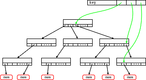
Pay attention again to Figure 1. This intermediate graph can be represented by a binary tree built on the principle of the Radix Tree (or the Russian equivalent - the tree of residues). Let's take a closer look at this data structure.

Adding an item to Radix Tree is as follows:
- Every i-th bit of the added value is taken.
- The element is pushed down the tree, based on the current bit. If the i-th bit is 0, then we go to the left, otherwise to the right.
And so on until all significant bits of the value have been processed.
- As a result, the Radix Tree leaf node will denote the value itself. So, going from the root to the leaf node,
get all the bits of the value. An illustration of the approach can be found here . In the Russian wiki description of the Radix Tree yet.

For example, take three numbers: 0123, 01234, 123 . Then at the first iteration, the tree is built from top to bottom, creating 4 nodes (0,1,2,3-leaf). In the second iteration, when adding the number 01234, we will follow the same path when adding the elements 0, 1, 2 and 3, since the nodes for these numbers have already been created. But when adding the last element, being in the node with a value of 3, we create a new leaf node 4. And at the third iteration, adding the number 123, the right side occurs.

If we present the obtained tree as a graph, where the node on the right is a “brother” and the node on the left is a “son”, we get the following picture

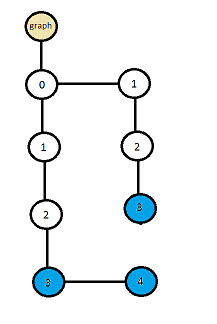
Figure 3. Link graph

Apply the add algorithm to Radix Tree for our extended graph. The graph node is represented by an array of 12 possible values ​​(0-9 * #). That is, we use the expandedNode [digit] mapping to check and set the node value.
In the figure below, expandedGraph is represented as an array of nodes expandedNode. '-' indicates an empty element, blue - indicates a leaf node. Let me remind you that the leaf node in our task contains number attributes.


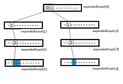
Figure 4. Extended (uncompressed) graph

I think the idea of ​​using Radix Tree is becoming clearer and from the picture itself it is clear that compression can be done by removing empty elements.

Compression. Building a compact graph.

The compression algorithm is relatively simple, and can be described in two sentences. We have an expanded graph of expandedGraph, represented as an array from expandedNode.
- We take non-empty elements (numbers) from the node expandedGraph [i]. We transfer them to a compressed graph, which is represented by an array of SG_Y_CompactNode. Set the length of a compact node as the number of non-empty elements.
- Apply a compression procedure for each child node. Changing links to child elements relative to the beginning of CompactGraph.

The compression algorithm is recursive. We select non-empty elements from the node, and lay them out sequentially in a compressed graph, specifying the length of the node. Thus, from the extended view node
"01 -----------" we get a compact node '[2] 01', where [2] is the length of the node.
Recursively call the procedure for the child elements '0' and '1'. Then we associate '0' and '1' with the children relative to the beginning of the squeezed graph.


Figure 5. The result is a compressed graph.

Conclusion

- The use of the algorithm is best suited for compressing and storing phone numbers. Prefixes like codes of mobile operators , country or city codes , allow to store these codes in the root nodes of the graph. The implementation is directly used in the software of a large telecommunications company.
However, it can be used for any data sequences. For example, to store Latin character data without case-sensitive, the size of a graph node must be increased to 26 elements. Accordingly, under the digit field, select 5 bits.
If attributes are not required, then the size of SG_Y_DigitElement can be reduced up to 2 bytes. For example, 5 bits for a character value, 10 bits for a pointer to the next node, and 1 bit for a sheet marker.
Obviously, restrictions on the number of addressable entries are limited to the nextNodeOffset field. In our example, 13 bits is enough to address 8192 entries.

Here is the implementation of the algorithm