Chalk-cepstral coefficients (MFCC) and speech recognition
Recently I came across an interesting article published by rgen3 , which describes the DTW-speech recognition algorithm. In general terms, this is a comparison of speech sequences using dynamic programming.
Interested in the topic, I tried to apply this algorithm in practice, but in this way I waited for a number of rakes. First of all, what exactly needs to be compared? Directly sound signals in the time domain are long and not very effective. Spectrograms are faster, but not much more efficient. The search for the most rational representation led me to the MFCC or the Chalk-frequency cepstral coefficients, which are often used as a characteristic of speech signals. Here I will try to explain what they are.
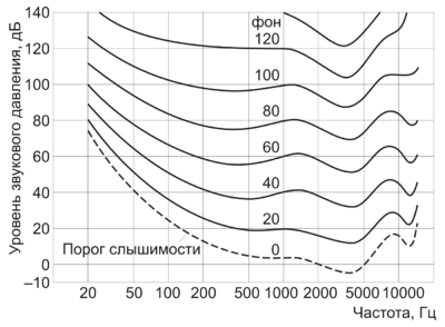
The explanation will start with the first word in the title. What is chalk? Wikipedia tells us that chalk is a unit of pitch based on the perception of this sound by our organs of hearing. As you know, the frequency response of the human ear does not even remotely resemble a straight line, and the amplitude is not an entirely accurate measure of the volume of the sound. Therefore, empirically selected units of volume were introduced, for example, background .
Similarly, the pitch of the sound perceived by human hearing does not quite linearly depend on its frequency.
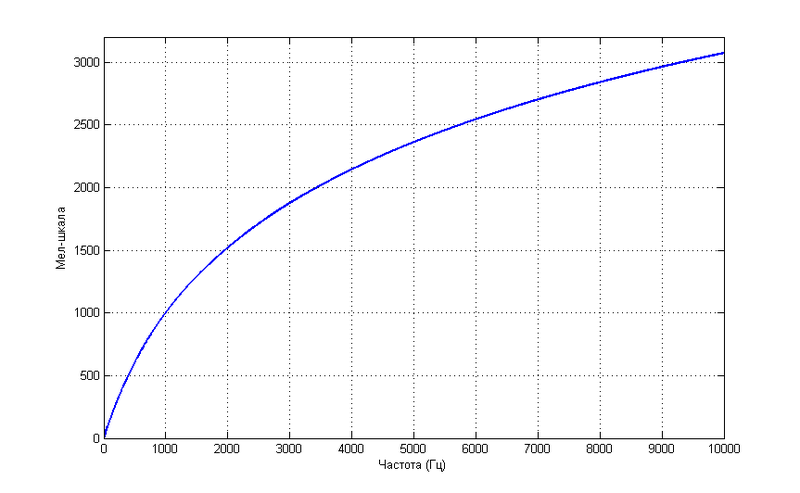
Such a dependence does not claim to be more accurate, but is described by a simple formula

')
Such units of measure are often used in solving problems of recognition, as they allow you to get closer to the mechanisms of human perception, which is still leading among the well-known speech recognition systems.
It is necessary to tell a little about the second word in the title - kepstrum .
In accordance with the theory of speech production, speech is an acoustic wave that is emitted by a system of organs: the lungs, bronchi and trachea, and then is transformed in the vocal tract. If we assume that the sources of excitation and the shape of the vocal tract are relatively independent, the human speech apparatus can be represented as a set of tonal and noise generators, as well as filters. Schematically it can be represented as follows:

1. Pulse sequence generator (tones)
2. The random number generator (noise)
3. Digital filter coefficients (voice path parameters)
4. Non-stationary digital filter
The signal at the output of the filter (4) can be represented in the form of convolution

where s (t) is the initial form of the acoustic wave, and h (t) is the filter characteristic (depends on the parameters of the vocal tract)
In the frequency domain, it looks like this

The work can be calibrated to get the amount instead.

Now we need to convert this sum so as to obtain non-overlapping sets of characteristics of the original signal and filter. There are several options for this, for example, the inverse Fourier transform will give us this

Also, depending on the target, you can use the direct Fourier transform or the discrete cosine transform
I hope I clarified the basic concepts a little. It remains to understand how to convert a speech signal into a set of MFCC coefficients.
As an experimental, we take a simple figure 1, here is its temporary representation
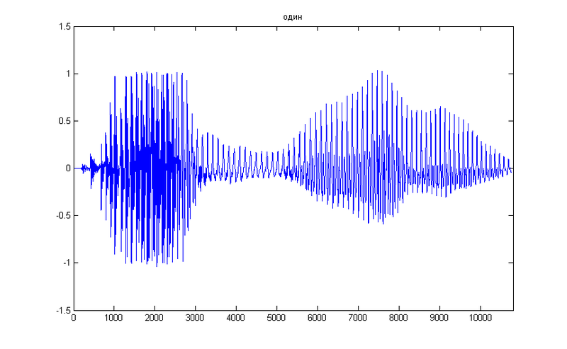
First of all, we need the spectrum of the original signal, which we obtain using the Fourier transform . For simplicity of the example, we will not break the signal into parts, therefore we take the spectrum along the entire time axis

Now the most interesting begins, we need to place the resulting spectrum on a chalk scale. For this, we use windows evenly spaced on the chalk axis.

If you translate this graph into a frequency scale, you can see such a picture

On this graph, it is noticeable that the windows are “collected” in the low-frequency region, providing a higher “resolution” where it is necessary for recognition.
By a simple multiplication of the vectors of the signal spectrum and the window function, we find the energy of the signal that falls into each of the analysis windows. We received a certain set of coefficients, but these are not the MFCCs we are looking for. While they could be called Mel-frequency spectral coefficients. We square them and logarithmize them. It remains for us to only get one of them cepstral, or "spectrum spectrum." For this, we could once again apply the Fourier transform, but it is better to use the discrete cosine transform .
As a result, we obtain a sequence of approximately the following form:

Thus, we have a very small set of values, which, when recognized, successfully replaces thousands of samples of the speech signal. They write in the books that it is possible to take the first 13 of the 24 calculated coefficients for the word recognition problem, but in my case any suitable results started from 16. In any case, this is a much smaller amount of data than the spectrogram or the temporal representation of the signal.
For best results, you can split the source word into short lengths, and calculate the coefficients for each of them. “Weighting” window functions can also help. It all depends on the recognition algorithm to which you feed the result.
I do not want to load the main part of the article with a large number of formulas, but suddenly they will be interesting to someone. Therefore, I will bring them here.
The original speech signal is written in discrete form as
Apply the Fourier transform to it.
We make a combination of filters using the window function

For which the frequency f [m] is obtained from the equation

B (b) - conversion of the frequency value into a chalk scale, respectively,

We calculate energy for each window

Apply DCT

We receive the MFCC set
[1] Wikipedia
[2] Xuedong Huang, Alex Acero, Hsiao-Wuen Hon, Spoken Language Processing, Algorithm, System Development, Prentice Hall, 2001, ISBN: 0130226165
Interested in the topic, I tried to apply this algorithm in practice, but in this way I waited for a number of rakes. First of all, what exactly needs to be compared? Directly sound signals in the time domain are long and not very effective. Spectrograms are faster, but not much more efficient. The search for the most rational representation led me to the MFCC or the Chalk-frequency cepstral coefficients, which are often used as a characteristic of speech signals. Here I will try to explain what they are.
Basic concepts
The explanation will start with the first word in the title. What is chalk? Wikipedia tells us that chalk is a unit of pitch based on the perception of this sound by our organs of hearing. As you know, the frequency response of the human ear does not even remotely resemble a straight line, and the amplitude is not an entirely accurate measure of the volume of the sound. Therefore, empirically selected units of volume were introduced, for example, background .
Similarly, the pitch of the sound perceived by human hearing does not quite linearly depend on its frequency.
Such a dependence does not claim to be more accurate, but is described by a simple formula
')
Such units of measure are often used in solving problems of recognition, as they allow you to get closer to the mechanisms of human perception, which is still leading among the well-known speech recognition systems.
It is necessary to tell a little about the second word in the title - kepstrum .
In accordance with the theory of speech production, speech is an acoustic wave that is emitted by a system of organs: the lungs, bronchi and trachea, and then is transformed in the vocal tract. If we assume that the sources of excitation and the shape of the vocal tract are relatively independent, the human speech apparatus can be represented as a set of tonal and noise generators, as well as filters. Schematically it can be represented as follows:
1. Pulse sequence generator (tones)
2. The random number generator (noise)
3. Digital filter coefficients (voice path parameters)
4. Non-stationary digital filter
The signal at the output of the filter (4) can be represented in the form of convolution
where s (t) is the initial form of the acoustic wave, and h (t) is the filter characteristic (depends on the parameters of the vocal tract)
In the frequency domain, it looks like this
The work can be calibrated to get the amount instead.
Now we need to convert this sum so as to obtain non-overlapping sets of characteristics of the original signal and filter. There are several options for this, for example, the inverse Fourier transform will give us this
Also, depending on the target, you can use the direct Fourier transform or the discrete cosine transform
I hope I clarified the basic concepts a little. It remains to understand how to convert a speech signal into a set of MFCC coefficients.
Example
As an experimental, we take a simple figure 1, here is its temporary representation
First of all, we need the spectrum of the original signal, which we obtain using the Fourier transform . For simplicity of the example, we will not break the signal into parts, therefore we take the spectrum along the entire time axis
Now the most interesting begins, we need to place the resulting spectrum on a chalk scale. For this, we use windows evenly spaced on the chalk axis.
If you translate this graph into a frequency scale, you can see such a picture
On this graph, it is noticeable that the windows are “collected” in the low-frequency region, providing a higher “resolution” where it is necessary for recognition.
By a simple multiplication of the vectors of the signal spectrum and the window function, we find the energy of the signal that falls into each of the analysis windows. We received a certain set of coefficients, but these are not the MFCCs we are looking for. While they could be called Mel-frequency spectral coefficients. We square them and logarithmize them. It remains for us to only get one of them cepstral, or "spectrum spectrum." For this, we could once again apply the Fourier transform, but it is better to use the discrete cosine transform .
As a result, we obtain a sequence of approximately the following form:
Conclusion
Thus, we have a very small set of values, which, when recognized, successfully replaces thousands of samples of the speech signal. They write in the books that it is possible to take the first 13 of the 24 calculated coefficients for the word recognition problem, but in my case any suitable results started from 16. In any case, this is a much smaller amount of data than the spectrogram or the temporal representation of the signal.
For best results, you can split the source word into short lengths, and calculate the coefficients for each of them. “Weighting” window functions can also help. It all depends on the recognition algorithm to which you feed the result.
Formulas
I do not want to load the main part of the article with a large number of formulas, but suddenly they will be interesting to someone. Therefore, I will bring them here.
The original speech signal is written in discrete form as
Apply the Fourier transform to it.
We make a combination of filters using the window function
For which the frequency f [m] is obtained from the equation
B (b) - conversion of the frequency value into a chalk scale, respectively,
We calculate energy for each window
Apply DCT
We receive the MFCC set
Sources
[1] Wikipedia
[2] Xuedong Huang, Alex Acero, Hsiao-Wuen Hon, Spoken Language Processing, Algorithm, System Development, Prentice Hall, 2001, ISBN: 0130226165
Source: https://habr.com/ru/post/140828/
All Articles