What is the role of the first "random" layer in the Rosenblatt perceptron
So in the article by Perceptron Rosenblatt - what is forgotten and invented by history? in principle, as expected, some lack of awareness of the essence of Rosenblatt's perceptron has surfaced (someone has more, someone has less). But honestly, I thought it would be worse. Therefore, for those who are able and willing to listen, I promised to write how it turns out that random links in the first layer perform such a complex task of displaying a non-separable (linearly not separable) representation of the problem into a separable (linearly separable).
Honestly, I could just refer to the Rosenblatt convergence theorem, but since I do not like it when they “send me to Google,” let's understand. But I proceed from the fact that you know from the originals what Rosenblatt’s perceptron is (although problems in understanding have surfaced, but I still hope that only certain people).
')
Let's start with the materiel
So the first thing we need to know is what the perceptron A matrix is and the perceptron G matrix. I give references to Wikipedia, I wrote myself therefore you can trust (directly from the original):
1. A-matrix perceptron
2. G-matrix of the perceptron , here it is necessary to pay attention to the Relationship of A and G - the perceptron matrices
who will not master this, please do not read further, close the article and smoke - this article is not for you. Do not rush, not everything in life at once becomes clear, it also took me a couple of years to study the nuances of the perceptron. Read here a little - do experiments.
Next, let's talk about the theory of perceptron convergence. There is a lot of talk about her, but I am sure that 50% have never seen her.
So, from one of my scientific articles:
I naturally will not consider the evidence (see the original), but what will be important to us later is that the perceptron convergence is not mathematically guaranteed (it will not be guaranteed, it will not be with simple input data, even if it is broken, it is about arbitrary input data) in two cases:
1. If the number of examples in the training sample is greater than the number of neurons in the middle layer (A-elements)
2. If the determinant is zero for the G matrix
In the first part, everything is simple, we can always set the number of A-elements equal to the number of examples in the training set.
But the second part is especially interesting in the light of our question. If you have coped with the understanding of what this G-matrix is, then it is clear that it depends on the input data and on what connections were formed by chance in the first layer.
And now we come to the question:
The probability of activity of A - elements
Next, I'll skip the details a bit and give the drawing immediately:
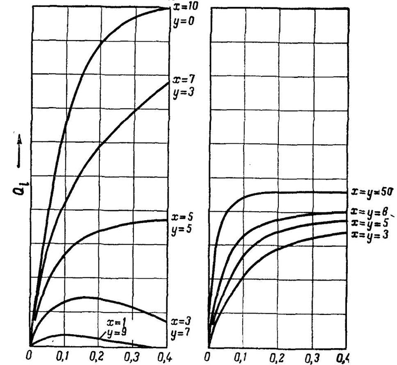
this is so-called Q-functions analyzed by Rosenblatt. I will not go into details, but here it is important that:
x is the number of excitatory connections in the first layer, matching one A-element (weight +1) and y the number of inhibiting (weight -1). Along the y axis, the figure shows the value of this Q-function, which depends on the relative number of illuminated elements on the retina (1 at the input).
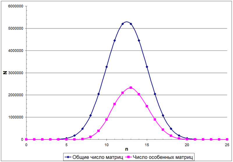
And in this case the number of units in the matrix A will be described by the binomial distribution. For example, the following figure shows the distribution of the number of matrices N depending on the number of units n in the matrix, 5x5 in size
And finally, what is the probability that a matrix is special?
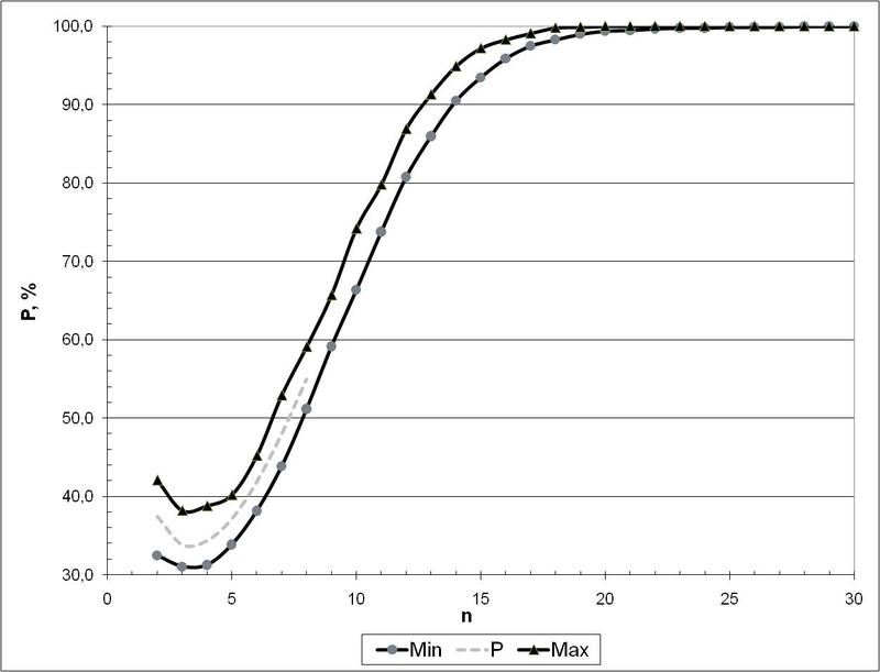
And this is what you see in the following figure (these are the probabilities of the appearance of non- special matrices depending on their size):
So, it is clear from this that even with a matrix size of 30 x 30 (that is, when the number of A-elements is 30 or more), it can be said that there is almost 100% certainty that the randomly obtained matrix will not be special. This is the final practical condition under which the Rosenblatt perceptron will form a space that satisfies the compactness hypothesis. It is practically safer to have a minimum of about 100 A-elements to exclude the case when the G-matrix becomes special.
In conclusion. Now ask yourself: does the MLP + BackProp guarantee what I have stated to you here regarding the Rosenblatt perceptron? I haven’t found any convincing evidence of this anywhere (just don’t throw links to the material. Proof of the convergence of the gradient descent - this does not apply, my opponents are best advised to write my own intelligible article on this subject: " thoughts from your head are welcome in Habrahabr " more constructive). But based on the problem of hitting the local minima when using BackProp - it seems that not everything is clean and smooth, as with Rosenblatt's perceptron.
upd. which I missed a little in the presentation, and during the dialogue we clarified here. Thank you retran and justserega for the leading questions.
Summary. In corollaries 1 and 2, it is stated that in certain conditions a solution is impossible. Here I proved that such conditions do not occur for n> 30 (Rosenblatt did not deal with this). But readers have two questions.
1. Good A-matrix (and through it, and G) is suitable with high probability. But how does this help move to another space? . Indeed, not very obvious. I explain. The A-matrix is the “other space” - the space of signs. The fact that the matrix is not special and that this matrix is one dimension larger than the original one is a sign that it can be divided linearly. (this follows from the corollaries and Theorem 3)
2. " Is there any evidence that the error correction algorithm in the Rosenblatt perceptron will converge? ". Indeed, Theorem 3 says only that a solution exists. This already means that this solution exists in the feature space, i.e. after working a random first layer. The error correction algorithm teaches the second layer, and Rosenblatt has Theorem 4, in which he proves that existing possible solutions (Theorem 3, that they exist at all) can be achieved precisely by applying the learning algorithm with error correction.
Another important point follows from the fact that the A-matrix depends, on the one hand, on the input data and, on the other hand, on the random matrix of relations. More precisely, the input matrix is mapped into the matrix A through a random operator (randomly formed bonds). If we introduce the measure of randomness, as the rate of occurrence of subsequences that will be repeated (pseudo-randomness), it turns out: (1) if this is not an accidental at all, but an operator constructed according to certain rules (i.e., the first layer connection), the probability of getting And -matrix is special (2) if, after multiplying the input matrix by the pseudo-randomness we obtained, the A-matrix has not a regular, but a chaotic scatter of units (let's call this condition R) - then this is exactly what we analyzed above.
Here I will reveal to you the tried and tested thing. According to the idea of a binomial randomness model when creating connections (this is when an A-element is taken and N exciting and M inhibiting connections to S-elements are randomly carried out from it) to satisfy condition R. But to speed up the convergence process, you can get a greater level of chaos Matrix A. How to do it - cryptography just tells us. This is the connection with cryptography.
Honestly, I could just refer to the Rosenblatt convergence theorem, but since I do not like it when they “send me to Google,” let's understand. But I proceed from the fact that you know from the originals what Rosenblatt’s perceptron is (although problems in understanding have surfaced, but I still hope that only certain people).
')
Let's start with the materiel
So the first thing we need to know is what the perceptron A matrix is and the perceptron G matrix. I give references to Wikipedia, I wrote myself therefore you can trust (directly from the original):
1. A-matrix perceptron
2. G-matrix of the perceptron , here it is necessary to pay attention to the Relationship of A and G - the perceptron matrices
who will not master this, please do not read further, close the article and smoke - this article is not for you. Do not rush, not everything in life at once becomes clear, it also took me a couple of years to study the nuances of the perceptron. Read here a little - do experiments.
Next, let's talk about the theory of perceptron convergence. There is a lot of talk about her, but I am sure that 50% have never seen her.
So, from one of my scientific articles:
The following theorem was proved:
“'' Theorem 3. '' An elementary perceptron, the stimulus space W and some classification C (W) are given. Then for the existence of a solution, it is necessary and sufficient that there exists some vector u lying in the same orthant as C (W) and some vector x such that Gx = u. "
as well as two direct consequences of this theorem:
“'' Corollary 1. '' The elementary perceptron and the stimulus space W are given. Then, if G is a special matrix (whose determinant is zero), then there is some classification C (W) for which there is no solution.”
“'' Corollary 2. '' If the number of stimuli in the space W is greater than the number A - of the elements of the elementary perceptron, then there exists a certain classification C (W) for which there is no solution”.
Rosenblatt calls the stimulus space the source data space.
I naturally will not consider the evidence (see the original), but what will be important to us later is that the perceptron convergence is not mathematically guaranteed (it will not be guaranteed, it will not be with simple input data, even if it is broken, it is about arbitrary input data) in two cases:
1. If the number of examples in the training sample is greater than the number of neurons in the middle layer (A-elements)
2. If the determinant is zero for the G matrix
In the first part, everything is simple, we can always set the number of A-elements equal to the number of examples in the training set.
But the second part is especially interesting in the light of our question. If you have coped with the understanding of what this G-matrix is, then it is clear that it depends on the input data and on what connections were formed by chance in the first layer.
And now we come to the question:
But since the first layer of connections in the perceptron is chosen randomly and is not trained, it is often thought that with equal probability the perceptron may or may not work with linearly inseparable source data, and only linear source data guarantee its flawless operation. In other words, the matrix of the perceptron with equal probability can be both special and not special. Here it will be shown that this opinion is wrong. (here and further, quotes from my scientific articles)
The probability of activity of A - elements
From the definition of the matrix A we see that it is binary, and takes the value 1 when the corresponding A is active. We will be interested in what is the probability of a unit appearing in the matrix and, accordingly, what is the probability of zero.
Next, I'll skip the details a bit and give the drawing immediately:
this is so-called Q-functions analyzed by Rosenblatt. I will not go into details, but here it is important that:
x is the number of excitatory connections in the first layer, matching one A-element (weight +1) and y the number of inhibiting (weight -1). Along the y axis, the figure shows the value of this Q-function, which depends on the relative number of illuminated elements on the retina (1 at the input).
The figure shows the dependence of the activity probability of the A - element Qi on the magnitude of the illuminated area of the retina. Note that for models that have only exciting connections (y = 0) with a high number of illuminated S - elements, the value of Qi approaches 1. That is, the probability of activity of A - elements is directly dependent on the number of illuminated S - elements, which is bad affects the recognition of relatively small and large images. As will be shown below, this is due to the high probability that the A-matrix will be special. Therefore, for the stability of pattern recognition of any geometrical dimensions, it is necessary to choose the ratio x: y so that the probability of activity of the A elements as low as possible depends on the number of illuminated S elements.
... it can be seen that for x = y, the value of Qi remains approximately constant throughout the entire region, except for a very small or very large number of illuminated S - elements. And if you increase the total number of bonds, the area in which Qi remains constant expands. When the threshold is small and x and y are equal, the value approaches 0.5, i.e. equal to the likely occurrence of A-element activity on an arbitrary stimulus . Thus, conditions are found under which the appearance of a unit and zero in matrix A is equiprobable.
And in this case the number of units in the matrix A will be described by the binomial distribution. For example, the following figure shows the distribution of the number of matrices N depending on the number of units n in the matrix, 5x5 in size
And finally, what is the probability that a matrix is special?
From the binomial distribution, you can find out how the total number of matrices with different number of units in the matrix is distributed (the upper curve in the previous figure). But for the number of non-singular matrices (lower curve in the previous figure) the mathematical formula does not currently exist.
But there is a sequence A055165 [6], which gives the probability of precisely the fact that the nxn matrix is not special. But it can be calculated only by enumeration and this is done before the cases of n <= 8. But subsequent values can be obtained by the Monte Carlo method ...
And this is what you see in the following figure (these are the probabilities of the appearance of non- special matrices depending on their size):
So, it is clear from this that even with a matrix size of 30 x 30 (that is, when the number of A-elements is 30 or more), it can be said that there is almost 100% certainty that the randomly obtained matrix will not be special. This is the final practical condition under which the Rosenblatt perceptron will form a space that satisfies the compactness hypothesis. It is practically safer to have a minimum of about 100 A-elements to exclude the case when the G-matrix becomes special.
In conclusion. Now ask yourself: does the MLP + BackProp guarantee what I have stated to you here regarding the Rosenblatt perceptron? I haven’t found any convincing evidence of this anywhere (just don’t throw links to the material. Proof of the convergence of the gradient descent - this does not apply, my opponents are best advised to write my own intelligible article on this subject: " thoughts from your head are welcome in Habrahabr " more constructive). But based on the problem of hitting the local minima when using BackProp - it seems that not everything is clean and smooth, as with Rosenblatt's perceptron.
upd. which I missed a little in the presentation, and during the dialogue we clarified here. Thank you retran and justserega for the leading questions.
Summary. In corollaries 1 and 2, it is stated that in certain conditions a solution is impossible. Here I proved that such conditions do not occur for n> 30 (Rosenblatt did not deal with this). But readers have two questions.
1. Good A-matrix (and through it, and G) is suitable with high probability. But how does this help move to another space? . Indeed, not very obvious. I explain. The A-matrix is the “other space” - the space of signs. The fact that the matrix is not special and that this matrix is one dimension larger than the original one is a sign that it can be divided linearly. (this follows from the corollaries and Theorem 3)
2. " Is there any evidence that the error correction algorithm in the Rosenblatt perceptron will converge? ". Indeed, Theorem 3 says only that a solution exists. This already means that this solution exists in the feature space, i.e. after working a random first layer. The error correction algorithm teaches the second layer, and Rosenblatt has Theorem 4, in which he proves that existing possible solutions (Theorem 3, that they exist at all) can be achieved precisely by applying the learning algorithm with error correction.
Another important point follows from the fact that the A-matrix depends, on the one hand, on the input data and, on the other hand, on the random matrix of relations. More precisely, the input matrix is mapped into the matrix A through a random operator (randomly formed bonds). If we introduce the measure of randomness, as the rate of occurrence of subsequences that will be repeated (pseudo-randomness), it turns out: (1) if this is not an accidental at all, but an operator constructed according to certain rules (i.e., the first layer connection), the probability of getting And -matrix is special (2) if, after multiplying the input matrix by the pseudo-randomness we obtained, the A-matrix has not a regular, but a chaotic scatter of units (let's call this condition R) - then this is exactly what we analyzed above.
Here I will reveal to you the tried and tested thing. According to the idea of a binomial randomness model when creating connections (this is when an A-element is taken and N exciting and M inhibiting connections to S-elements are randomly carried out from it) to satisfy condition R. But to speed up the convergence process, you can get a greater level of chaos Matrix A. How to do it - cryptography just tells us. This is the connection with cryptography.
Source: https://habr.com/ru/post/140387/
All Articles