Recommended systems: user-based and item-based
So, last time we talked a little about what recommender systems are all about and what problems they face, and also about what the formulation of the collaborative filtering problem looks like. Today I will talk about one of the simplest and most natural methods of collaborative filtering, from which research in this area began in the 90s. The basic idea is very simple: how to understand whether Vasya will like the film “Tractor drivers”? You just need to find other users similar to Vasya, and see what ratings they put on “Tractor drivers”. Or on the other hand: how to understand whether Vasya likes the film “Tractor Drivers”? You just need to find other films similar to "Tractor Drivers" and see how Vasya evaluated them.
Let me remind you that we have a very sparse matrix consisting of ratings (likes, purchase facts, etc.) that users (matrix rows) assigned to products (matrix columns):

Our task is to predict estimates. knowing some of the ratings already placed in the matrix
  . Our best prediction will be denoted by
  . If we can get these predictions, we just need to select one or more products for which maximum.
We mentioned two approaches: either look for similar users — this is called “user-based collaborative filtering”, or look for similar products — that is logical, called “product-based recommendations” (item-based collaborative filtering). Actually, the basic algorithm in both cases is clear.
It remains only to understand how to do it all.
')
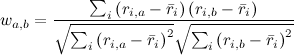
First, you need to determine what “similar” means. I remind you that all we have is a vector of preferences for each user (rows of the R matrix) and a vector of user ratings for each product (columns of the R matrix). First of all, we leave in these vectors only those elements for which we know the values in both vectors, i.e. Leave only those products that are rated by both users, or only those users who both rate this product. As a result, we just need to determine how similar the two vectors of real numbers are. This is, of course, a well-known problem, and its classical solution is to calculate the correlation coefficient: for two user preference vectors i and j, the Pearson correlation coefficient is
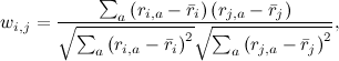
Where - average rating given by user i. Sometimes they use the so-called "cosine similarity" using the cosine of the angle between the vectors:
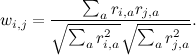
But in order for the cosine to work well, it is advisable to still first subtract the average for each vector, so in reality it is the same metric.
For example, consider some evaluation matrix.
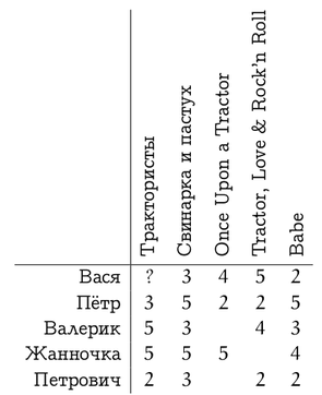
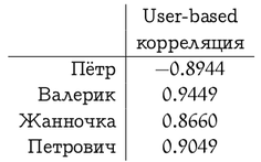
We will leave the manual analysis of preferences to the reader, and calculate for the user-based recommendations the correlation between the preference vector of Vasya and the rest of the participants in the system.
We have now given formulas for user-based recommendations. In the item-based approach, the situation is similar, but there is one nuance: different users relate differently to the estimates, someone puts everyone in a row with five asterisks (websites like "like"), and someone, on the contrary, puts everything in two or three stars (often shakes "dizlike"). For the first user, a low rating (“dizlink”) will be much more informative than a high one, and for the second, the opposite. In the user-based approach, the correlation coefficient automatically takes care of this. And in the item-based recommendations, to take this into account, you can, for example, subtract the average rating of a particular user from each assessment, and then calculate the correlation or cosine of the angle between the vectors. Then in the formula for the cosine we get
 ,
,
Where denotes the average rating given by user i. In our example, if you subtract the average from each vector of estimates, you get this:

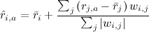
And then the correlation between the ratings vector of the film “Tractorists” and the ratings of other films will be (note that a degenerate situation has developed with “Once Upon a Tractor” because there were too few overlapping assessments)
These measures of similarity have their drawbacks and various variations on the theme, but for the illustration of the methods let us limit ourselves to them. Thus, we have dealt with the first point of the plan; Next in line is the second - how to use these similarity estimates (weights )?
)?
A simple and logical approach is to bring a new rating as the average rating of a given user plus deviations from the average ratings of other users weighed by these weights:
 .
.
This approach is sometimes also called the GroupLens algorithm - this is how the grandfather of the GroupLens recommender systems worked (by the way, pardon the pun, I recommend MovieLens site] - serious collaborative filtering actually started with it once, but today it can please little-known films that you like) . In the case of Vasya and Tractor Engineers, this method is expected to have a rating of about 3.9 (Petrovich let us down a little), so you can safely look.
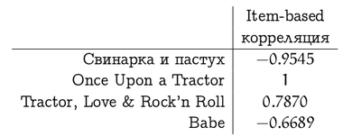
For item-based recommendations, everything is absolutely equivalent - you just need to find the weighted average of the products already rated by the user:

The item-based method in our example assumes that Vasya will deliver to "Tractor Engineers" 4.4.
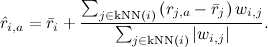
Of course, theoretically all this is good, but in reality it is unlikely for each recommendation to summarize the data from millions of users. Therefore, this formula is usually roughed up to k nearest neighbors - k users who are as similar as possible to this user and have already evaluated this product:
It remains only to understand how to quickly find the nearest neighbors. This is already beyond the scope of our discussion, so I’ll just call two main methods: in small dimensions, you can use kd-trees (kd-trees, see, for example, this introduction ), and in large dimensions you can use locally sensitive hashing (locally sensitive). hashing, see, for example, here ).
So, today we have considered the simplest recommender algorithms that evaluate the similarity of a user (product) to other users (other products), and then recommend, based on the opinion of the closest neighbors in this metric. By the way, one should not think that these methods are completely outdated - for many problems they work perfectly. However, in the next series, we turn to a more subtle analysis of the available information. In particular, from the very beginning I persistently called the input data a “rating matrix,” although it would seem that we never used the fact that it is really a matrix, and not just a set of vectors (either rows or columns, depending on the method). Next time - use.
PS For images with formulas, thanks to the mathURL service. Unfortunately, he does not understand Russian letters, so the tables about Vasya and Petrovich had to be made by hand.
Let me remind you that we have a very sparse matrix consisting of ratings (likes, purchase facts, etc.) that users (matrix rows) assigned to products (matrix columns):
Our task is to predict estimates.
knowing some of the ratings already placed in the matrix . Our best prediction will be denoted by . If we can get these predictions, we just need to select one or more products for which maximum.We mentioned two approaches: either look for similar users — this is called “user-based collaborative filtering”, or look for similar products — that is logical, called “product-based recommendations” (item-based collaborative filtering). Actually, the basic algorithm in both cases is clear.
- Find how other users (products) in the database are similar to this user (product).
- It is estimated by other users (products) to predict what rating this user will give to this product, given the greater weight of those users (products) that are more similar to this one.
It remains only to understand how to do it all.
')
First, you need to determine what “similar” means. I remind you that all we have is a vector of preferences for each user (rows of the R matrix) and a vector of user ratings for each product (columns of the R matrix). First of all, we leave in these vectors only those elements for which we know the values in both vectors, i.e. Leave only those products that are rated by both users, or only those users who both rate this product. As a result, we just need to determine how similar the two vectors of real numbers are. This is, of course, a well-known problem, and its classical solution is to calculate the correlation coefficient: for two user preference vectors i and j, the Pearson correlation coefficient is
Where
- average rating given by user i. Sometimes they use the so-called "cosine similarity" using the cosine of the angle between the vectors:But in order for the cosine to work well, it is advisable to still first subtract the average for each vector, so in reality it is the same metric.
For example, consider some evaluation matrix.
We will leave the manual analysis of preferences to the reader, and calculate for the user-based recommendations the correlation between the preference vector of Vasya and the rest of the participants in the system.
We have now given formulas for user-based recommendations. In the item-based approach, the situation is similar, but there is one nuance: different users relate differently to the estimates, someone puts everyone in a row with five asterisks (websites like "like"), and someone, on the contrary, puts everything in two or three stars (often shakes "dizlike"). For the first user, a low rating (“dizlink”) will be much more informative than a high one, and for the second, the opposite. In the user-based approach, the correlation coefficient automatically takes care of this. And in the item-based recommendations, to take this into account, you can, for example, subtract the average rating of a particular user from each assessment, and then calculate the correlation or cosine of the angle between the vectors. Then in the formula for the cosine we get
,Where
denotes the average rating given by user i. In our example, if you subtract the average from each vector of estimates, you get this:And then the correlation between the ratings vector of the film “Tractorists” and the ratings of other films will be (note that a degenerate situation has developed with “Once Upon a Tractor” because there were too few overlapping assessments)
These measures of similarity have their drawbacks and various variations on the theme, but for the illustration of the methods let us limit ourselves to them. Thus, we have dealt with the first point of the plan; Next in line is the second - how to use these similarity estimates (weights
)?A simple and logical approach is to bring a new rating as the average rating of a given user plus deviations from the average ratings of other users weighed by these weights:
.This approach is sometimes also called the GroupLens algorithm - this is how the grandfather of the GroupLens recommender systems worked (by the way, pardon the pun, I recommend MovieLens site] - serious collaborative filtering actually started with it once, but today it can please little-known films that you like) . In the case of Vasya and Tractor Engineers, this method is expected to have a rating of about 3.9 (Petrovich let us down a little), so you can safely look.
For item-based recommendations, everything is absolutely equivalent - you just need to find the weighted average of the products already rated by the user:
The item-based method in our example assumes that Vasya will deliver to "Tractor Engineers" 4.4.
Of course, theoretically all this is good, but in reality it is unlikely for each recommendation to summarize the data from millions of users. Therefore, this formula is usually roughed up to k nearest neighbors - k users who are as similar as possible to this user and have already evaluated this product:
It remains only to understand how to quickly find the nearest neighbors. This is already beyond the scope of our discussion, so I’ll just call two main methods: in small dimensions, you can use kd-trees (kd-trees, see, for example, this introduction ), and in large dimensions you can use locally sensitive hashing (locally sensitive). hashing, see, for example, here ).
So, today we have considered the simplest recommender algorithms that evaluate the similarity of a user (product) to other users (other products), and then recommend, based on the opinion of the closest neighbors in this metric. By the way, one should not think that these methods are completely outdated - for many problems they work perfectly. However, in the next series, we turn to a more subtle analysis of the available information. In particular, from the very beginning I persistently called the input data a “rating matrix,” although it would seem that we never used the fact that it is really a matrix, and not just a set of vectors (either rows or columns, depending on the method). Next time - use.
PS For images with formulas, thanks to the mathURL service. Unfortunately, he does not understand Russian letters, so the tables about Vasya and Petrovich had to be made by hand.
Source: https://habr.com/ru/post/139518/
All Articles