Comparison of compression programs as applied to transferring large amounts of data
It all started with a simple task: download a large amount of data on a 100-megabit network using
After that, there was a question about the analysis of the applicability of common compression programs.
for data transmission over the network.
The first task was to collect baseline data for analysis. Experimental choices fell on common compression programs in the * nix world. All programs were installed from standard Ubuntu 11.10 repositories:
')
Official sites: lzop , gzip , bzip2 , xz .
bzip2 is based on the BWT algorithm ( English ), the rest are based on the LZ77 algorithm ( English ) and its modifications.
For lzop, compression ratios of 2-6 are identical and therefore not tested.
The test system was a laptop on the Intel P8600 (Core 2 Duo, 2.4 GHz)
c 4 GB of RAM, running under Ubuntu 11.10 64-bit.
For testing used several different data sets:
Well, more "classic" sets:
The measurement technique was as follows: for each program, the compression ratio, and the source file, compression was performed into an intermediate file with time measurement, then the size of the compressed file was remembered,
then unpacking was performed with time measurement. Just in case, the unpacked file was compared with the original one, then the intermediate and unpacked files were deleted.
To eliminate the effect of disk I / O on the results, all files were placed in
Each measurement was carried out 3 times. As a result, a minimum time of three was used.
The results are shown in charts in the coordinates of the packing time - the size of the packaged file.
Fig. 1: Graph of results for gcc compiler source codes:

Fig. 2: Graph of the results for a binary distribution of ParaView:
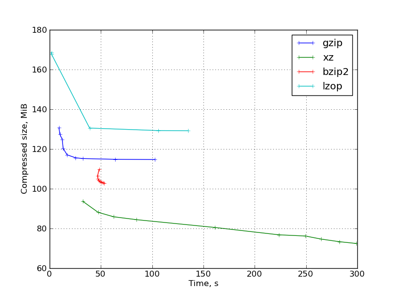
Fig. 3: Graph of results for a binary scientific data set:
Also graphics for: kernel headers and OpenFoam source code .
Consider this scenario of data transmission over the network: first, the data is packaged, then transmitted over the network, then unpacked. Then the total time will be:
where
This equation defines a constant time curve in the graphs shown, the slope of which is determined by the network bandwidth. To determine the optimal packing algorithm for a given bandwidth, you need to find the lowest straight line with the desired slope passing through any point of the graph.
That is, the optimal methods of compression and the speed of their “switching” are determined by the lines tangent to our set of points on the graph. It remains only to determine them.
What we are looking for is nothing more than a convex hull ( born convex hull). Numerous algorithms have been developed for constructing the convex hull of a set of points. I used implementation on python from here .
After constructing the convex hull, the points belonging to it will be our optimal algorithms, and the slopes of the edges connecting them will be the boundary capacities.
Thus we obtain the following optimal algorithms for our files:
Now consider another scenario: the data is packed, and immediately as it is sent, it is sent over the network, and on the receiving side it is immediately unpacked.
Then the total data transfer time is determined not by the sum, but by the maximum of three times: packaging, unpacking, and transmission over the network.
The constant time curve for the selected network bandwidth will then look like an angle with apex on a straight line
and two rays going down and to the left from the top.
Algorithm that allows you to find all the best methods of compression and boundary bandwidths, in this case is much easier. First we sort the points by time, then we select the first optimal point (this will be a point without compression, with zero time. The absence of compression is optimal for a network of infinite capacity.) Now we are going through the points in the order of increasing compression time. If the file size is smaller than the file size of the previous optimal method, then the current method becomes the new optimal one. In this case, the boundary bandwidth will be equal to the file size of the previous method divided by the compression time of the new method.
Here are the results for this use case:

It is known that one of the fastest channels for delivering large amounts of information over short distances is a cycle courier with hard drives.
Count. Let the distance be 10 kilometers. The cyclist will make a round-trip flight in an hour and a half (at a normal pace and taking into account any delays, loading and unloading) Let it give 6 flights per 8-hour working day. Let him take with him 10 drives of 1 TB. Then he will transport 60 TB per day. This is equivalent to round-the-clock operation of a line with a throughput of 60 TB / (24 * 3600) with = 662 MiB / s, which is approximately 5 Gbit / s. Not bad.
The results show that if you try to compress the data for such a communication line on one core, similar to the cores of my laptop, then the absence of compression is optimal.
And if we consider the case of transferring data on a single USB 2.0 hard drive, then this is similar to scenario 2 with a speed of approximately 30 MB / s, if we consider the time costs only on the transmitting side.
Looking at our graph, we get:
If we first compress and then copy to an external disk, then this is scenario 1, and then
rsync . The question arose whether this process could be accelerated. The top utility showed that on the source server, encryption takes up no more than 10 percent of the processor, so it was decided that you could try data compression. At that time, it was unclear to me whether processor performance would be enough to pack data at the required speed, so the smallest compression ratio was set, namely the --compress-level=1 flag was used for rsync . It turned out that the processor load did not exceed 65%, that is, the processor performance was enough, while the speed of downloading the data somewhat increased.After that, there was a question about the analysis of the applicability of common compression programs.
for data transmission over the network.
Source Data Collection
The first task was to collect baseline data for analysis. Experimental choices fell on common compression programs in the * nix world. All programs were installed from standard Ubuntu 11.10 repositories:
')
  Program Version Test Keys Default
 lzop 1.03 1, 3, 7-9 3
 gzip 1.3.12 1-9 6
 bzip2 1.0.5 1-9 9
 xz 5.0.0 0-9 7
Official sites: lzop , gzip , bzip2 , xz .
bzip2 is based on the BWT algorithm ( English ), the rest are based on the LZ77 algorithm ( English ) and its modifications.
For lzop, compression ratios of 2-6 are identical and therefore not tested.
The test system was a laptop on the Intel P8600 (Core 2 Duo, 2.4 GHz)
c 4 GB of RAM, running under Ubuntu 11.10 64-bit.
For testing used several different data sets:
- The source code of a large C ++ project openfoam.com , packaged in a tar. It contains source code, documentation in pdf, and a certain amount of poorly compressible scientific data.
Uncompressed volume: 127641600 bytes = 122 MiB - The binary distribution of a large project paraview.org , packaged in a tar. Consists mainly of .so library files.
Uncompressed volume: 392028160 bytes = 374 MiB - Binary scientific data set.
Uncompressed volume: 151367680 bytes = 145 MiB
Well, more "classic" sets:
- Linux kernel headers, packaged in tar.
Uncompressed volume: 56657920 bytes = 55 MiB - The gcc compiler source code, packaged in tar.
Uncompressed volume: 490035200 bytes = 468 MiB
The measurement technique was as follows: for each program, the compression ratio, and the source file, compression was performed into an intermediate file with time measurement, then the size of the compressed file was remembered,
then unpacking was performed with time measurement. Just in case, the unpacked file was compared with the original one, then the intermediate and unpacked files were deleted.
To eliminate the effect of disk I / O on the results, all files were placed in
/run/shm (this is shared memory in linux, with which you can work as with the file system).Each measurement was carried out 3 times. As a result, a minimum time of three was used.
Measurement results
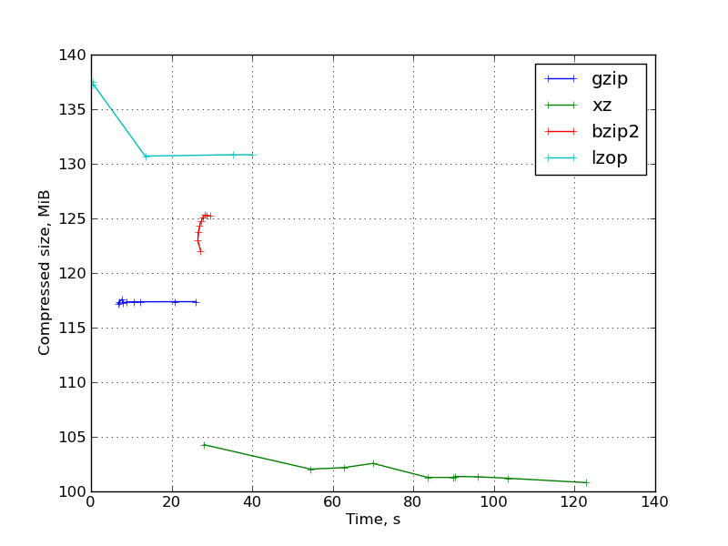
The results are shown in charts in the coordinates of the packing time - the size of the packaged file.
Fig. 1: Graph of results for gcc compiler source codes:
Fig. 2: Graph of the results for a binary distribution of ParaView:
Fig. 3: Graph of results for a binary scientific data set:
Also graphics for: kernel headers and OpenFoam source code .
Observations:
- With compression rates of 7-9, lzop becomes very slow without a large reduction in file size, and loses much more than gzip. These lzop compression ratios are completely useless.
With the default compression level, lzop is, as expected, very fast. The compression ratio -1 does not give a big time gain, giving a larger file size. - gzip behaves as expected. "Correct" form of the graph when changing the degree of compression.
- bzip2 was not very competitive. In most cases, it loses both in compression ratio and speed in low compression ratios xz. The exceptions are the kernel headers and gcc source code (that is, purely textual information) on which they compete. In this light, it is rather strange that bzip2 on the Internet is much more popular than xz. This is probably due to the fact that the second is rather young and has not yet become an “standard” one.
It is also worth noting that different keys change the compression ratio and the bzip2 operation time is very small. - xz at large values of the parameter shows a high degree of compression, but at the same time it works very slowly and requires a very large amount of memory for compression (approximately 690 MB at -9, the required memory size is indicated in man). The size of the memory for unpacking is significantly less, but it can still be
restriction for some applications.
Small compression ratios closely approach gzip -9 in runtime, providing a better compression ratio.
In general, you can see that xz gives a fairly large selection of ratios of compression ratio and time. - Unpacking of LZ-77-based programs occurs fairly quickly, and with an increase in the compression ratio (within the same program), the unpacking time decreases slightly.
With bzip2, unpacking is slower, and the unpacking time increases with increasing compression.
Analysis: Scenario 1 — Sequential Operations
Consider this scenario of data transmission over the network: first, the data is packaged, then transmitted over the network, then unpacked. Then the total time will be:
t = t_c + s / bw + t_d
where
t_c is the packing time, s is the packed file size in bytes, bw is the network bandwidth in bytes / s, t_d is the unpacking time.This equation defines a constant time curve in the graphs shown, the slope of which is determined by the network bandwidth. To determine the optimal packing algorithm for a given bandwidth, you need to find the lowest straight line with the desired slope passing through any point of the graph.
That is, the optimal methods of compression and the speed of their “switching” are determined by the lines tangent to our set of points on the graph. It remains only to determine them.
What we are looking for is nothing more than a convex hull ( born convex hull). Numerous algorithms have been developed for constructing the convex hull of a set of points. I used implementation on python from here .
After constructing the convex hull, the points belonging to it will be our optimal algorithms, and the slopes of the edges connecting them will be the boundary capacities.
Thus we obtain the following optimal algorithms for our files:
Analysis: Scenario 2 - Stream Compression
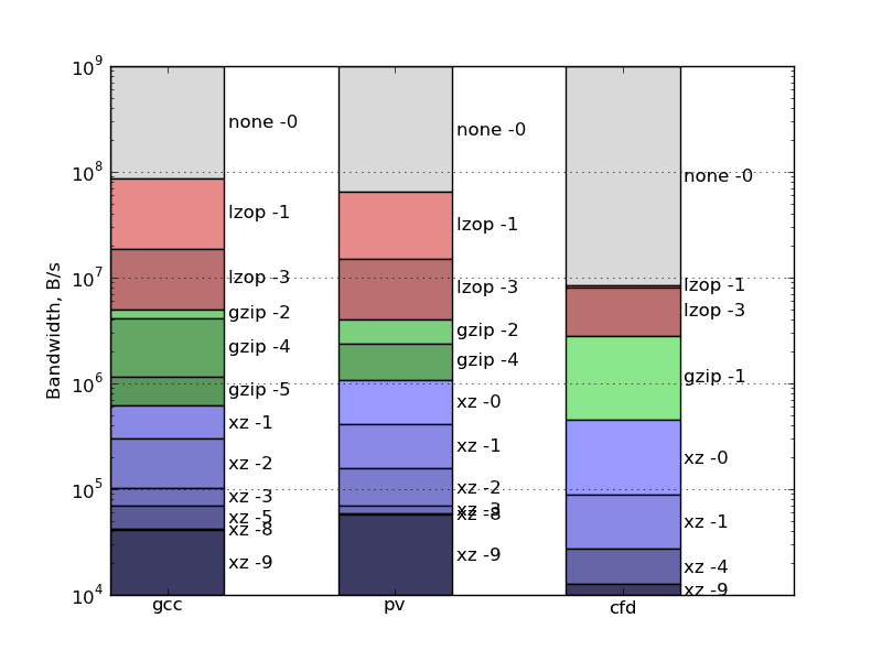
Now consider another scenario: the data is packed, and immediately as it is sent, it is sent over the network, and on the receiving side it is immediately unpacked.
Then the total data transfer time is determined not by the sum, but by the maximum of three times: packaging, unpacking, and transmission over the network.
The constant time curve for the selected network bandwidth will then look like an angle with apex on a straight line
t = s / bw
and two rays going down and to the left from the top.
Algorithm that allows you to find all the best methods of compression and boundary bandwidths, in this case is much easier. First we sort the points by time, then we select the first optimal point (this will be a point without compression, with zero time. The absence of compression is optimal for a network of infinite capacity.) Now we are going through the points in the order of increasing compression time. If the file size is smaller than the file size of the previous optimal method, then the current method becomes the new optimal one. In this case, the boundary bandwidth will be equal to the file size of the previous method divided by the compression time of the new method.
Here are the results for this use case:
Final notes
- Everything written concerns only scenarios with the transmission of large amounts of data, and does not apply to other scenarios, for example, with the transmission of many small messages.
- This study had a model character and does not pretend to fully take into account all the features arising in real life. Here are some of them:
- Disk I / O is not considered.
- The presence and possibility of using multiple processor cores is not taken into account.
- It does not take into account that in a server application, there may be another load on the processor at the same time, leaving less resources for compression.
- This study does not include snappy from google. It happened for several reasons.
- First of all, it does not have a native command line utility (in fact, there is a third-party snzip , but I do not think that it can be considered any standard).
- Secondly, it is intended for other applications.
- Thirdly, it promises to be even faster than lzop, which means that it can be very difficult to correctly measure its operation time.
Practical examples
It is known that one of the fastest channels for delivering large amounts of information over short distances is a cycle courier with hard drives.
Count. Let the distance be 10 kilometers. The cyclist will make a round-trip flight in an hour and a half (at a normal pace and taking into account any delays, loading and unloading) Let it give 6 flights per 8-hour working day. Let him take with him 10 drives of 1 TB. Then he will transport 60 TB per day. This is equivalent to round-the-clock operation of a line with a throughput of 60 TB / (24 * 3600) with = 662 MiB / s, which is approximately 5 Gbit / s. Not bad.
The results show that if you try to compress the data for such a communication line on one core, similar to the cores of my laptop, then the absence of compression is optimal.
And if we consider the case of transferring data on a single USB 2.0 hard drive, then this is similar to scenario 2 with a speed of approximately 30 MB / s, if we consider the time costs only on the transmitting side.
Looking at our graph, we get:
lzop -3 is optimal for transferring data on an external USB hard drive for our test datasets.If we first compress and then copy to an external disk, then this is scenario 1, and then
lzop -1 turns out to be optimal in terms of total time consumption for source codes and binary distribution, and for poorly compressible binary data - no compression.Additional links
- Similar comparison: http://stephane.lesimple.fr/wiki/blog/lzop_vs_compress_vs_gzip_vs_bzip2_vs_lzma_vs_lzma2-xz_benchmark_reloaded
- Another comparison: http://www.linuxjournal.com/node/8051/
Source: https://habr.com/ru/post/139012/
All Articles