In previous articles ( 1 , 2 ) we got acquainted with how the data may look depending on the biological experiment performed. Based on these visualized data, assumptions were made about what happens inside the cell. Now we will focus on how to mathematically and algorithmically analyze the data so that the machines for us can perform the routine work. Unfortunately, after reading a lot of articles on data analysis, I got the impression that there is no unambiguous or most universal solution. There are algorithms that show themselves well on a certain set of data, and in other cases no longer respond to the tasks set.

First I want to remind you and explain a little the basic concepts used in the article. Every time I talk about the reads, and how they are produced, I come across surprising and misunderstanding. And then by chance, throwing a pack of paper in a shredder, I understood how to try to explain what reads are. Suppose you have a book, the book itself is a cell, and each chapter of the book is DNA. You already have several million copies of this book. You fed the books to the shredder, which cut them into strips. Here you take a container with nakromsannymi paper strips, mix them well and take out what the first one got. Next, carefully lay out the strips, from both sides cut into small pieces and put the cut pieces in a separate box. These little pieces are reads, the strips are fragments. Further, with the help of a certain program, we determine in which part of the book the cut piece was located. Sometimes we get lucky and we can pinpoint the place in the book where the piece was cut from. Sometimes the program identifies several possible locations for this piece, for example, due to the fact that some chapters began with a repetition of the previous one or as a result of all operations some letters were erased and they were not found in the book. The number of variations on the topic that could happen with pieces of strips is very large, if you can discuss them all, you can not get to the algorithms. I hope, now it has become clearer what is what.

Describing the algorithm, I will talk about it, using the data on which the developers tested it. But this does not mean that it cannot be used on data of another type. I will also try to identify the shortcomings of the algorithms that I encountered. I do not attempt to systematize the algorithms; I will describe them in groups, in the order in which they were used in the general analysis of the sequenced data. In this article I will talk about a simple analysis of “pollution by the adapter” and about the preliminary preparation of the landscape and, probably, in the next article or through one - about assessing the quality of the data obtained.


')

Contamination adapter

Companies producing equipment for sequencing also produce related kits: slides, tubes, reagents. One type of reagent is the polynucleotide chain necessary for sequencing, which is called an adapter.

There are various types of contamination of the prepared material. One of them is pollution by the adapter. The analysis of such pollution is simple. It is necessary to calculate the frequency of nucleotides on the first, second, etc. positions of the received FASTA / FASTQ file. Based on the data obtained, a table is compiled. Consider the analysis process in more detail, using the following example, below are the first 9 columns of the table (see Table 1):

Table 1

Pos / Nucl	0	one	2	3	four	five	6	7
A	446500	2869138	599400	941816	1145756	1133404	3599581	3291736
C	1922795	1367021	1761361	3723679	1030494	1173573	963827	1284534
T	485441	1337742	3273475	918001	1016981	1006168	1494250	1291715
G	4130093	1425977	1365764	1416504	3806769	3686855	942342	1132015
N	15171	122

Using the data table, you can build a graph (Fig. 1). The peaks of the graph correspond to the letter (nucleotide) most frequently found at the current position. In particular, the letter “G” in the first, the letter “A” in the second, “T” in the third position.


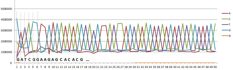
Fig. one


If you make up the entire chain of letters corresponding to the peaks, you get a sequence that is most often found in the original data. If this sequence coincided with the sequence from the list of adapters (which are supplied by manufacturers of equipment for sequencing), as for example, in the considered example, one of the Illumina adapter sequences was obtained, then the adapter was contaminated.

To calculate the percentage of pollution adapter and the source material, perform the following simple steps. 1. We count the total number of letters in one of the positions in the table, in the given example, they are exactly 7000000. 2. If there was no contamination, then the number of letters in each position should be approximately the same. Excluding from consideration the letter corresponding to the peak, we consider the rest. As follows from the graph, there are about 1,200,000 such letters in each position. 3. Since there must be the same number of letters in each position, we get: 1,200,000 * 4 = 4,800,000. 4. Thus, the adapter's pollution is: 4,800,000 / 7,000,000 * 100% = 32%. Those. when preparing the material the next time you need to reduce the number of added adapters.

Preparing a profile for further analysis

Most of the algorithms known to me perform the initial data processing - they prepare a profile. That is, group the data, and then evaluate their level of significance. The grouped data will determine the location of the likely location of the protein on the DNA that we are trying to find using algorithms.

Consider the data resulting from the use of chromatin immunoprecipitation (for more details, “ DNA Sequencing ”). Let me remind you about the features of this method: fragments are selected using antibodies corresponding to the proteins of interest, as a result, most fragments contain the sequence to which the protein was attached. Also, when cutting, fragments of different size are obtained, they are additionally filtered in length (no more than 150-300 nucleotides). Most of the reads are ultimately located on both sides of the protein. This feature we will use in the future to determine the likely location of the protein.


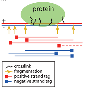
Fig. 2


In Figure 2, the yellow arrows show the possible locations of the DNA cut, this is where fragments can begin or end. Red lines depict reads obtained from a positive helix (indicated with a “+” sign), and blue lines show a negative helix (indicated by a “-” sign). In some cases, if a more expensive experiment is performed (“ pair-end sequencing ”), the sequencing equipment is able to determine which two reads were obtained from a single fragment. It is also stated that the use of such a method several times increases the quality of determining the proposed position of a protein [1]. The pair-end method is still not used frequently, so in most cases we are dealing with an unrelated set of reads.

In the ideal case, the landscape of the location of the reads around the protein should be as in Figure 3. Given that the possible number of random components of the experiment is large, this is rare.


Fig. 3


Below are examples of landscapes from experimental data (Fig. 4). The width of the column (window) corresponds to 20 nucleotides, the maximum height of the columns is only 5-8 reads. If the width of the window were equal to one nucleotide, then the image would become even more discrete and noisy. But, if the data are processed using the profile preparation algorithms proposed below, the landscape will be more like the ideal one (Fig. 3).


Fig. four

Manual profile preparation

How to bring the data to a more readable form for the machine? In some cases, we know in advance how long fragments are expected. For example, in the case of H3K4Me3 (MNase method), they are about 148bp [2]. Shift the reads by half the fragment length: 148/2 = 74. The reads found on the positive spiral are shifted to the right by 74, found on the negative spiral, shifted to the left by 74. Add the absolute values ​​and display on the graph (Fig. 5) [3, four].


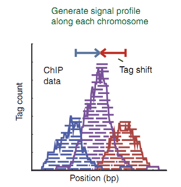
Fig. five

In the figure (Fig. 5), the peak in purple is displayed as a result of adding the number of reads from the positive and negative sides of the spiral. The top of the peak should correspond with some accuracy to the center of the location of the protein on the DNA. With such a simple transformation, we amplified the signal, and now it should become more noticeable.

There are various ways of plotting the graphs above. One of the ways: along the “Y” axis, we postpone the number of reads originating at the “X” point. Another way: plotting using segments, along the “Y” axis, we postpone the number of read crossings at a given “X” point. Sometimes a graph is built, setting off along the “Y” axis the intersection not of reads, but of fragments. The meaning of such graphs is the density of DNA coverage with reads / fragments.

This is good when you can estimate the fragment size in advance and transfer its value to the program. But what to do if the fragment length is not known, how can we calculate the value by which the data must be shifted?

Cross-correlation training profile

One way to calculate the magnitude of the shift is to cross-correlate read data from a positive and negative helix. For each chromosome “c” we define the function , which takes at each point “x” a value equal to the number of beginnings on the side of the helix “s”. Define for shear function 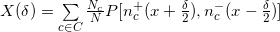where:

• - linear Pearson coefficient between vectors “a” and “b”;
• C - a set of all chromosomes;
• N _c is the number of reads on the “c” chromosome;
• N is the total number of reads.

Choose a range in which there can be a shift value, for example, from -100 to 300 and construct a graph (Fig. 6) [4].


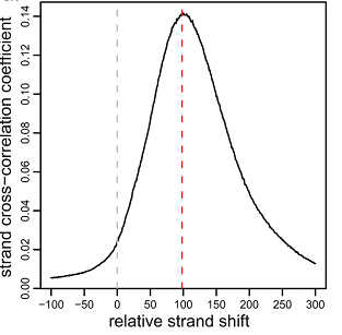
Fig. 6


The peak of this graph along the “x” axis will correspond to the shift with the highest correlation. In the case shown in Figure 6, the shift is 100/2 = 50 nucleotides. The correlation of data with all chromosomes may be less accurate with respect to the correlation of the area of ​​interest. So get their shear for each enriched segment.

Kernel density profile

Consider the algorithm using the kernel density functions [4,5,6]. Redefine the coverage density for each position i in accordance with the formula 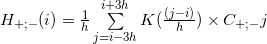where:

• h - kernel density bandwidth, in article [5] 30bp was used, and in article [4] they took 0.45 of the width of the peak in the middle, shown in Figure 6;
• - Gaussian kernel density function;
• - returns the number of reads that ended at point j on the positive and negative spiral, respectively.

Thus, having recalculated the density for each helix and amplifying the signal, for well-enriched areas we can determine the peaks on each side of the helix and take half the difference between them for the shift value (Fig. 7, “Peak shift”).


Fig. 7

Geometric profile building method

This algorithm uses simple mathematical operations. For a window wide in w and for position i, we define: p1 (i), as the number of tags in the window on the positive spiral to the left of i; p2 (i), as the number of tags to the right of position i. We define n1 (i) and n2 (i) according to the definition of p, only for the negative spiral (Fig. 8.1). Calculate the value at point i using the following formula: within the specified window we find the maximum. The maximum found is the estimated sticking position of the protein. This method is called WTD from Windows Tag Density.
In article [4] he was also offered to modify where P [a, b] is the linear Pearson correlation coefficient between vectors a and b, such that, vector “a” is the number of reads on the positive helix from position i to i + k, and vector “b” is the number Reads on the negative helix from position i to ik, (Figure 8.2). Called MTC from Mirrow Tag Correlation.




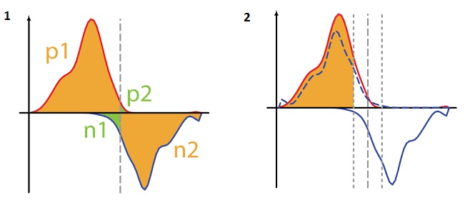
Fig. eight


There are other algorithms used in the construction of the profile [7]. I tried to highlight the most frequently used. All algorithms already have an implementation in any software package, links are given in articles, here are some of them:
sissrs.rajajothi.com
http://home.gwu.edu/~wpeng/Software.htm
mendel.stanford.edu/sidowlab/downloads/quest
http://compbio.med.harvard.edu/software.html .

Proper construction of a profile with the help of algorithms is the most important part of all programs, because the more precisely it is built, the more likely it is to determine where the protein is located. Another part of the algorithms is aimed at mathematically estimating how significant the found sections are. But, unfortunately, all algorithms are not able to replace a person, and can only help in the routine processing of data, hinting at the place where you should search. So while the whole system of interaction of biology, chemistry, mathematics and programming is far from perfect, and there is a huge field for searching, implementing and improving ideas.

1. Wang, C., et al., An effective approach for protein in vivo protein-DNA binding sites from ChIP-Seq data. BMC Bioinformatics, 2010. 11: p. 81. www.ncbi.nlm.nih.gov/pmc/articles/PMC2831849

2. Barski, A., et al., High-resolution profiling of the human genome. Cell, 2007. 129 (4): p. 823-37. www.ncbi.nlm.nih.gov/pubmed/17512414

3. Pepke, S., B. Wold, and A. Mortazavi, Computation for ChIP-seq and RNA-seq studies. Nat Methods, 2009. 6 (11 Suppl): p. S22-32. www.ncbi.nlm.nih.gov/pubmed/19844228

4. Kharchenko, PV, MY Tolstorukov, and PJ Park, ChIP-seq experiments for DNA-binding proteins. Nat Biotechnol, 2008. 26 (12): p. 1351-9. www.ncbi.nlm.nih.gov/pubmed/19029915

5. Valouev, A., et al., Genome-wide analysis of transcription factor binding sites based on ChIP-Seq data. Nat Methods, 2008. 5 (9): p. 829-34. www.ncbi.nlm.nih.gov/pubmed/19160518

6. Boyle, AP, et al., F-Seq: a feature density estimator for high-throughput sequence tags. Bioinformatics, 2008. 24 (21): p. 2537-8. www.ncbi.nlm.nih.gov/pmc/articles/PMC2732284

7. Zang, C., et al., A clustering approach for identification of enriched domains from histone modification ChIP-Seq data. Bioinformatics, 2009. 25 (15): p. 1952-8.

Some of the drawings were taken from nature.com and printed with their permission:
License Date: Feb 16, 2012,
License Numbers: 2850830942235, 2850831421638

Review by Andrey Kartashov, Covington, KY, porter@porter.st