The use of an inertial navigation system (INS) with several sensors on the example of the task of stabilizing the height of a quadrocopter
In this article I will try to talk about my experience in creating and implementing an algorithm for processing signals from several standard sensors that are part of the INS (in the English version of the IMU) to solve the problem of stabilizing the height of a multi-rotor aircraft (in my case, a quadrocopter). On Habré has already been a series of articles describing what kind of toy and how to make it yourself. As a programmer by profession, it was interesting for me not only to assemble him, but also to dig deeper into the “brains” and do something useful for the community. I chose Arduino and the wonderful MultiWii project as “brains”. It is completely open, dynamically developing, but so far there are “white spots” in it. For example, the stabilization of the position in height does not work satisfactorily. And I decided to find out whether it is possible to improve this part of the system with the available equipment.
First, some introductory information to clarify what is to be dealt with.
Multi-rotor is a device with several (3, 4, 6, 8) motors with propellers, each of which creates a vertical adjustable thrust. Unlike the helicopter, the stabilization here is completely electronic, and the microprocessor deals with it using the INS (flight controller).
')
At the moment, in easy accessibility we have a standard set of sensors:
Such a set complete with an Arduino-like processor or as a separate scarf can be found for a sum of $ 70-100
Each sensor has its own features and weaknesses. Individually, none of them can solve any of the problems listed above, so the INS systems are always built from a combination of sensors, and the most interesting thing here is computational algorithms that allow you to combine the strengths of each of the sensors to eliminate their shortcomings.
The first task, orientation stabilization, is quite successfully solved by gyroscopes. Gyroscopes measure the angular velocity very accurately and, after integration, angles can be obtained. But they have a problem - testimony floats with time. To correct this drift, an accelerometer is used, which always (or almost always in the long term) knows where the earth is. But the accelerometer will not feel anything if it is twisted around the Z axis, so we need a magnetometer, which always knows where the north is.
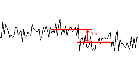
The second task - finding the height - is partially solved by a barometer. If we reset the readings on the ground, then when we climb every meter, we know how much his readings will change (naturally, if we don’t fly for 12 hours and the weather does not start changing). But according to the condition of the problem, the barometer is bad, and it gives out a height of + -1m with a wild noise amplitude approximately in the same range. In reality, my sensor shows the following (at the 10th second moved 1 meter):
Sonar can come to the aid of the barometer, which measures altitude with very high accuracy (even the one that I purchased for $ 5, gives an accuracy of ± 3mm according to the manufacturer). But the sonar is able to work only low above the ground (2-10m), measures for a long time (up to 200ms), is sensitive to the quality of the surface, to the angle of inclination, and can lose a signal.
The third task — determination of coordinates — is not solved by the sensors indicated above. Accelerometer in combination with a gyroscope can produce linear horizontal accelerations, but there are two problems here: a permanently large (compared to what we measure) vector 1G, and the lack of bindings for correction. So the determination of the coordinates remains the prerogative of the GPS-sensor, and one cannot count on high accuracy here.
In all amateur flight controllers, the problem of finding orientation has been solved well and I will not dwell on it. The task is quite simple and is written on the Internet ( one , two ). In MultiWii, a beautiful solution is used without complications such as quaternions and DCM matrices (do not forget that all this will be considered a simple 16 MHz processor), based on simplifications for small angles and a complementary filter.
So, we know the orientation of the apparatus in space with a high degree of accuracy. Now you can go to the main topic of the article, that is, try to improve the results that the barometer (or sonar) produces so that you can feed them to the PID controller . To do this, the readings must come without delay, be accurate in the short term, and not drift much over time. The topic of PID controllers deserves a separate close study, as it is widely used in process control systems. I recommend that you first familiarize yourself with their definition in order to better understand the reasoning set forth below.
What we do not fit the barometer readings in the current form? Well, firstly, a strong noise signal will cause unnecessary control actions on the motors. Applying a low pass filter, we reduce the noise, but lose the measurement speed. This means that any short-term perturbations will be ignored, sharp perturbations will be worked out with a long delay, and most importantly, we will not receive the differential component (D) for the PID controller. And as follows from the theory, a regulator without this component is prone to weakly damped oscillations around the target value, which is observed in practice.
Well, let's leave the barometer and take the accelerometer. It seems that everything is simple - from the value along the Z axis we subtract the constant 1G, we get linear vertical acceleration. We will integrate it twice (in fact, sum it up in the measuring cycle) and obtain the speed and relative displacement. For the PID controller, these are lacquered indicators, with them you can build a good dynamic model. But here, not everything is as good as we would like. The slope of the apparatus will cause a change in the projection of the acceleration vector A on the Z axis. Vibrations from the motor or temperature changes may cause a "shift" in sensitivity, and our constant 1G will no longer correspond to reality. But even in the case of a perfectly fixed device and a precisely exposed 1G, any sensor emits noise. But even a tiny mistake within a dozen seconds of double integration grows to the size of an elephant, and now we see a speed of 10m / s and a height of 20m (although they haven’t even come off the ground yet).
Explained in a simple way, this filter is applied to two values measured by different sensors and adjusts one of them so that it slowly approaches the second. In the measuring cycle, the filter is implemented with a simple formula:
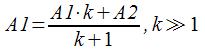
In this case, the effect of A2 on A1 is proportional to the difference between them and is determined by the coefficient k (the larger, the weaker the effect).
If you apply this filter to the height found by the accelerometer and the barometer readings, you get an interesting thing: the accelerometer drift will be constantly corrected by the barometer, and the barometer readings will be smoothed (since for A2 this filter works as a low-pass filter). But only the second integral will be adjusted, and the first will still quietly “drift” to infinity, and as a result, due to the small coefficient k, the barometer simply cannot influence the situation.
Why does this filter work fine for a pair of gyroscope + accelerometer? Because there we correct the first integral, and in the end it ceases to “float” when the correction value during one cycle equals the value of the gyroscope error added in the same cycle during integration.
But even from a pair of barometer + accelerometer, you can extract something useful if you apply a PID controller to them (yes, the area of their application is extremely extensive).
So what is the main weak point of our accelerator integrator? In a micro-error, which can occur for various reasons, as described above, when subtracting the constant 1G. If you write the desired acceleration in the form:
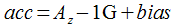
then, by adjusting the bias value, one can control both the first integral (velocity) and the second (offset). So, the goal of our PID controller is found. But you still need to know the error. Let us make the assumption that bias will be fixed after the onset of some stabilization of the system parameters (temperature, vibration, etc.). When bias is found, the accelerometer readings will be very close to the truth and you can apply a complementary filter, crossing them with a barometer. The magnitude of the correction of this filter will be an error from which the PID controller will repel (it seeks to reduce the error to 0 by adjusting the target variable).
Then we find all three components of the PID controller. Proportional (P) is the error itself. Integral (I) - just integrate it. Differential (D) - according to the theory it is necessary to differentiate the error. But there are terrible noises of the barometer and accelerometer. It's scary to differentiate this, so apply the trick - let's take the speed found by the accelerometer with a negative sign as the D-component. Since D is designed to introduce attenuation into the regulator, the speed here will fit perfectly - the more it is, the more it is necessary to “pay it off”.
Multiply each of the components by their coefficients, add and get bias. But here we apply the second trick - we will not add bias directly to the acceleration, but add only the I-part. It describes the magnitude of the permanent error, which corresponds to our assumption of a slow change in bias.
We add the P and D parts to the speed by multiplying by dT (since we borrowed them from acceleration).
Since the main task of the regulator is to find the constant component of the error, I decided to adjust it “softly” enough to minimize the short-term changes. But there remains a wide field for experiments, and everything will be determined by the behavior of real sensors.
Above, I mentioned that to determine the height, we also need a gyroscope. Indeed, the algorithm described above will work only if the vector A (in the local system) looks exactly along the Z axis. As soon as the device tilts, two unpleasant things will happen: the projection A on the Z axis will change and the PID controller will begin again slowly and painfully to search for bias . And the second - any horizontal acceleration will begin to give a non-zero projection on the local Z axis. At 45 ° tilt angles, you won’t understand where the acceleration is.
But since we know the exact orientation of the local system relative to the global, there is nothing difficult to restore justice - we simply design the local vector A onto the local vector G (originally found by the accelerometer and carefully rotated by the gyroscope), which always looks at the ground.
This operation is simple and follows from the definition of a vector product:

This must be done before subtracting 1G.
Now you can look at the code and the results.
Sensor data comes in the following variables:
EstG.V - vector G (it was obtained earlier while finding the orientation)
accADC - clean data from accelerometer
BaroAlt - data from the barometer, converted to cm
At the output we get accZ, vel, alt.
As you can see, the computational complexity of the algorithm is quite simple and Arduino will “digest” it easily (especially if translated into integer arithmetic, but then the code will become poorly readable).
PS: in the video there is a phrase about disabling the algorithm at a certain angle of inclination, and because of this, an error occurs. In fact, this restriction is not necessary - the algorithm works stably at any angle from 0 ° to 360 °
If you connect a sonar to this algorithm (in addition to BaroAlt, take SonarAlt), then the height curve looks almost perfect. Thus, at a low altitude we use sonar, when errors occur or close to the measurement limit, we switch to a barometer (having previously coordinated the altitudes in the period of receiving reliable data from the sonar).
Unfortunately, the weather does not allow to conduct flight tests of the new algorithm. As soon as the results appear, I'll post the sonar charts, the debugged source code of the entire project, and the flight video.
First, some introductory information to clarify what is to be dealt with.
Multi-rotor is a device with several (3, 4, 6, 8) motors with propellers, each of which creates a vertical adjustable thrust. Unlike the helicopter, the stabilization here is completely electronic, and the microprocessor deals with it using the INS (flight controller).
What tasks need to be solved in flight?
- Determination of orientation (angles along three axes relative to the ground) and stabilization along them
- Height determination and stabilization
- Determination of coordinates and flight at given points
- Receiving commands from the control panel and issuing control signals to the motors
')
What do we have available?
At the moment, in easy accessibility we have a standard set of sensors:
- pretty good 3-axis gyros.
- medium-quality 3-axis accelerometers
- medium quality 3-axis magnetometer
- medium or bad barometer
Such a set complete with an Arduino-like processor or as a separate scarf can be found for a sum of $ 70-100
Each sensor has its own features and weaknesses. Individually, none of them can solve any of the problems listed above, so the INS systems are always built from a combination of sensors, and the most interesting thing here is computational algorithms that allow you to combine the strengths of each of the sensors to eliminate their shortcomings.
The first task, orientation stabilization, is quite successfully solved by gyroscopes. Gyroscopes measure the angular velocity very accurately and, after integration, angles can be obtained. But they have a problem - testimony floats with time. To correct this drift, an accelerometer is used, which always (or almost always in the long term) knows where the earth is. But the accelerometer will not feel anything if it is twisted around the Z axis, so we need a magnetometer, which always knows where the north is.
The second task - finding the height - is partially solved by a barometer. If we reset the readings on the ground, then when we climb every meter, we know how much his readings will change (naturally, if we don’t fly for 12 hours and the weather does not start changing). But according to the condition of the problem, the barometer is bad, and it gives out a height of + -1m with a wild noise amplitude approximately in the same range. In reality, my sensor shows the following (at the 10th second moved 1 meter):
Sonar can come to the aid of the barometer, which measures altitude with very high accuracy (even the one that I purchased for $ 5, gives an accuracy of ± 3mm according to the manufacturer). But the sonar is able to work only low above the ground (2-10m), measures for a long time (up to 200ms), is sensitive to the quality of the surface, to the angle of inclination, and can lose a signal.
The third task — determination of coordinates — is not solved by the sensors indicated above. Accelerometer in combination with a gyroscope can produce linear horizontal accelerations, but there are two problems here: a permanently large (compared to what we measure) vector 1G, and the lack of bindings for correction. So the determination of the coordinates remains the prerogative of the GPS-sensor, and one cannot count on high accuracy here.
In all amateur flight controllers, the problem of finding orientation has been solved well and I will not dwell on it. The task is quite simple and is written on the Internet ( one , two ). In MultiWii, a beautiful solution is used without complications such as quaternions and DCM matrices (do not forget that all this will be considered a simple 16 MHz processor), based on simplifications for small angles and a complementary filter.
So, we know the orientation of the apparatus in space with a high degree of accuracy. Now you can go to the main topic of the article, that is, try to improve the results that the barometer (or sonar) produces so that you can feed them to the PID controller . To do this, the readings must come without delay, be accurate in the short term, and not drift much over time. The topic of PID controllers deserves a separate close study, as it is widely used in process control systems. I recommend that you first familiarize yourself with their definition in order to better understand the reasoning set forth below.
Smoothing
What we do not fit the barometer readings in the current form? Well, firstly, a strong noise signal will cause unnecessary control actions on the motors. Applying a low pass filter, we reduce the noise, but lose the measurement speed. This means that any short-term perturbations will be ignored, sharp perturbations will be worked out with a long delay, and most importantly, we will not receive the differential component (D) for the PID controller. And as follows from the theory, a regulator without this component is prone to weakly damped oscillations around the target value, which is observed in practice.
We integrate
Well, let's leave the barometer and take the accelerometer. It seems that everything is simple - from the value along the Z axis we subtract the constant 1G, we get linear vertical acceleration. We will integrate it twice (in fact, sum it up in the measuring cycle) and obtain the speed and relative displacement. For the PID controller, these are lacquered indicators, with them you can build a good dynamic model. But here, not everything is as good as we would like. The slope of the apparatus will cause a change in the projection of the acceleration vector A on the Z axis. Vibrations from the motor or temperature changes may cause a "shift" in sensitivity, and our constant 1G will no longer correspond to reality. But even in the case of a perfectly fixed device and a precisely exposed 1G, any sensor emits noise. But even a tiny mistake within a dozen seconds of double integration grows to the size of an elephant, and now we see a speed of 10m / s and a height of 20m (although they haven’t even come off the ground yet).
Complementary filter
Explained in a simple way, this filter is applied to two values measured by different sensors and adjusts one of them so that it slowly approaches the second. In the measuring cycle, the filter is implemented with a simple formula:
In this case, the effect of A2 on A1 is proportional to the difference between them and is determined by the coefficient k (the larger, the weaker the effect).
If you apply this filter to the height found by the accelerometer and the barometer readings, you get an interesting thing: the accelerometer drift will be constantly corrected by the barometer, and the barometer readings will be smoothed (since for A2 this filter works as a low-pass filter). But only the second integral will be adjusted, and the first will still quietly “drift” to infinity, and as a result, due to the small coefficient k, the barometer simply cannot influence the situation.
Why does this filter work fine for a pair of gyroscope + accelerometer? Because there we correct the first integral, and in the end it ceases to “float” when the correction value during one cycle equals the value of the gyroscope error added in the same cycle during integration.
PID controller comes to the rescue
But even from a pair of barometer + accelerometer, you can extract something useful if you apply a PID controller to them (yes, the area of their application is extremely extensive).
So what is the main weak point of our accelerator integrator? In a micro-error, which can occur for various reasons, as described above, when subtracting the constant 1G. If you write the desired acceleration in the form:
then, by adjusting the bias value, one can control both the first integral (velocity) and the second (offset). So, the goal of our PID controller is found. But you still need to know the error. Let us make the assumption that bias will be fixed after the onset of some stabilization of the system parameters (temperature, vibration, etc.). When bias is found, the accelerometer readings will be very close to the truth and you can apply a complementary filter, crossing them with a barometer. The magnitude of the correction of this filter will be an error from which the PID controller will repel (it seeks to reduce the error to 0 by adjusting the target variable).
Then we find all three components of the PID controller. Proportional (P) is the error itself. Integral (I) - just integrate it. Differential (D) - according to the theory it is necessary to differentiate the error. But there are terrible noises of the barometer and accelerometer. It's scary to differentiate this, so apply the trick - let's take the speed found by the accelerometer with a negative sign as the D-component. Since D is designed to introduce attenuation into the regulator, the speed here will fit perfectly - the more it is, the more it is necessary to “pay it off”.
Multiply each of the components by their coefficients, add and get bias. But here we apply the second trick - we will not add bias directly to the acceleration, but add only the I-part. It describes the magnitude of the permanent error, which corresponds to our assumption of a slow change in bias.
We add the P and D parts to the speed by multiplying by dT (since we borrowed them from acceleration).
Since the main task of the regulator is to find the constant component of the error, I decided to adjust it “softly” enough to minimize the short-term changes. But there remains a wide field for experiments, and everything will be determined by the behavior of real sensors.
But what about the gyroscope?
Above, I mentioned that to determine the height, we also need a gyroscope. Indeed, the algorithm described above will work only if the vector A (in the local system) looks exactly along the Z axis. As soon as the device tilts, two unpleasant things will happen: the projection A on the Z axis will change and the PID controller will begin again slowly and painfully to search for bias . And the second - any horizontal acceleration will begin to give a non-zero projection on the local Z axis. At 45 ° tilt angles, you won’t understand where the acceleration is.
But since we know the exact orientation of the local system relative to the global, there is nothing difficult to restore justice - we simply design the local vector A onto the local vector G (originally found by the accelerometer and carefully rotated by the gyroscope), which always looks at the ground.
This operation is simple and follows from the definition of a vector product:
This must be done before subtracting 1G.
Now you can look at the code and the results.
#define ACC_BARO_CMPF 300.0f #define ACC_BARO_P 30.0f #define ACC_BARO_I (ACC_BARO_P * 0.001f) #define ACC_BARO_D (ACC_BARO_P * 0.001f) #define VEL_SCALE ((1.0f — 1.0f/ACC_BARO_CMPF)/1000000.0f) #define ACC_SCALE 9.80665f / acc_1G / 10000.0f err = (alt - BaroAlt)/ACC_BARO_CMPF; // P term of error errI+= err * ACC_BARO_I; // I term of error accZ = (accADC[0]*EstG.VX + accADC[1]*EstG.VY + accADC[2]*EstG.VZ) * InvSqrt(fsq(EstG.VX) + fsq(EstG.VY) + fsq(EstG.VZ)) - errI - acc_1G; // Integrator - velocity, cm/sec vel+= (accZ - err*ACC_BARO_P - vel*ACC_BARO_D) * cycleTime * ACC_SCALE; // Integrator - altitude, cm alt+= vel * cycleTime * VEL_SCALE; // Apply ACC->BARO complementary filter alt-= err; errPrev = err; Sensor data comes in the following variables:
EstG.V - vector G (it was obtained earlier while finding the orientation)
accADC - clean data from accelerometer
BaroAlt - data from the barometer, converted to cm
At the output we get accZ, vel, alt.
As you can see, the computational complexity of the algorithm is quite simple and Arduino will “digest” it easily (especially if translated into integer arithmetic, but then the code will become poorly readable).
PS: in the video there is a phrase about disabling the algorithm at a certain angle of inclination, and because of this, an error occurs. In fact, this restriction is not necessary - the algorithm works stably at any angle from 0 ° to 360 °
If you connect a sonar to this algorithm (in addition to BaroAlt, take SonarAlt), then the height curve looks almost perfect. Thus, at a low altitude we use sonar, when errors occur or close to the measurement limit, we switch to a barometer (having previously coordinated the altitudes in the period of receiving reliable data from the sonar).
Unfortunately, the weather does not allow to conduct flight tests of the new algorithm. As soon as the results appear, I'll post the sonar charts, the debugged source code of the entire project, and the flight video.
Source: https://habr.com/ru/post/137595/
All Articles