Installation and initial setup of ZINBA

I noticed that the articles are quite large, and the questions are asked in different directions. This article was written to collect questions on installing the ZINBA program in a separate topic. So, to work with ZINBA, you need to know how to install it.


Detailed installation painted on the developer's site in English . Therefore, I will briefly describe the necessary steps in Russian. All the steps were performed by me in the OS OpenSUSE 12.1 x64, but must pass without incident on other Linux platforms. We start R (if there are questions on setup, we will discuss in comments), we execute the following commands:

• system ("wget zinba.googlecode.com/files/zinba_2.01.tar.gz "). Downloads the package from the developer’s site.
• install.packages (c ('multicore', 'doMC', 'foreach', 'qvalue', 'quantreg', 'R.utils')). Installs additional packages. A window will appear with a list of sites to download, select the site from which to install these packages.
• install.packages ("zinba_2.01.tar.gz", repos = NULL). The installation of the downloaded package occurs.

Now, after any launch of R, it is enough to run library (zinba) to activate the library. Further, it is recommended to perform the steps for initial configuration , namely:

• We go to the “Necessary file downloads” section, in the “Genome Build” subsection we download one or several two-bit genome indexes, it depends on which of them you are going to work with.
• In the subsection “Mappability files” we upload a file containing the name of the genome in the title and the length of the reads, as in your FASTA / FASTQ file. Do not forget to unzip it to any directory. In Linux, for example, you can download and unzip it like this: “wget www.bios.unc.edu/~nrashid/map##.tgz;tar -xzvf map ##. Tar.gz”, where ## is a number corresponding to the length reed
• Run R, execute two commands successively: 1. generateAlignability, to create an alignment index and 2. basealigncount, for a basic alignment count; This command will create a file containing the exact binding of the peaks in several iterations.

Further detailed description of these two commands:

generateAlignability( mapdir=, #   ,     «mappability» outdir=, #  ,      athresh=, # ,       extension=, #       twoBitFile=, #  ,    .2bit ) basealigncount( inputfile=, #      , ,  bowtie outputfile=, #   ,    extension=, #       filetype=, #   "bed", "bowtie", or "tagAlign" twoBitFile=, #   ,    .2bit ) 

The first command is recommended to be performed once and later only if the parameters of the experiments change, such as: the number of errors and the length of the fragments. The second command should be carried out from experiment to experiment, and then only if we need to improve the quality of finding enriched regions and peaks (as this requires additional computational load).
During the execution of these actions, I received a number of errors, talked with technical support. It turned out that I didn’t read the instructions well enough, and they didn’t have everything smoothly. First, if the file is received using a bowtie (the usual is not .sam, without the –S parameter), then the last column in the file should be simply removed, there should be 7 columns in the file. It also turned out that the separator is not only tabulation, but so make sure the fields do not contain spaces. This is true for version 2.01, promised to fix it in the future.
The team itself finding the enriched regions is described below, runs for a long time and eats up all the resources. I performed it on experimental data from 33.000.000 reads, on 4x CPUs (not to be confused with a stone, just 4 threads, one Core i7), 8Gb RAM, though in a VirtualBOX virtual machine, the calculations took 8 hours. If there is only 8Gb of RAM, I do not recommend putting more threads; the program will work more with the paging file than with the data.
')

 zinba( refinepeaks=, #   ( )? 1 -  , 0 -   seq=, #      input=, #     ,    ,   .    'none' filetype=, # : 'bed', 'bowtie',  'tagAlign' threshold=, #,    p value   .   ,  0.05 align=, #  ,   outdir   generateAlignability numProc=, # CPU   ,     ( Core i7  8,  7  ,   1) twoBit=, #  ,    .2bit outfile=, #      extension=, #       ###################   ################### basecountfile=, #  basecount ,   refinepeaks   1 broad=, # , TRUE  FALSE ( ) printFullOut=, #    : 1,   (  ); 0,   ( ) ) 

We have prepared the package for work, now is the time to launch something to check it. The developer offers a set of test files: http://www.unc.edu/~nur2/zinbaweb/test_data.tgz . In the command line consistently perform the following actions.

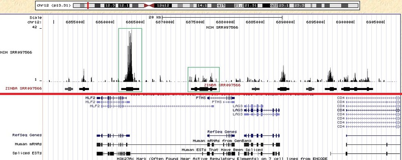
  # ,       . wget http://hgdownload.cse.ucsc.edu/goldenPath/hg19/bigZips/hg19.2bit wget http://www.bios.unc.edu/~nrashid/map36.tgz wget http://www.unc.edu/~nur2/zinbaweb/test_data.tgz #   tar -xzvf map36.tgz tar -xzvf test_data.tgz #   , , align_athresh1_extension200 mkdir align_athresh1_extension200 # R. R # R     library(zinba) generateAlignability( mapdir='map36/', outdir='align_athresh1_extension200/', athresh=1, extension=200, twoBitFile='hg18.2bit' ) basealigncount( inputfile='data/ctcfGM12878rep3chr22.taf', outputfile='data/ctcfGM12878rep3chr22.basecount', extension=200, filetype='tagAlign', twoBitFile='hg18.2bit' ) zinba( align='align_athresh1_extension200/', numProc=4, seq='data/ctcfGM12878rep3chr22.taf', basecountfile='data/ctcfGM12878rep3chr22.basecount', filetype="tagAlign", outfile="data/ctcf", twoBit="hg18.2bit", extension=200, printFullOut=1, refinepeaks=1, broad=F, input='data/inputGM12878rep3chr22.taf' ) 

In the data directory there will be files with the name ctcf and the extension .peaks, .peaks.bed, which contain the data of interest to us in the form of a table . The file with the .bed extension can be loaded into the genome browser and see.
I worked with other data taken from the NIH website www.ncbi.nlm.nih.gov/geo/roadmap/epigenomics , ftp-trace.ncbi.nlm.nih.gov/sra/sra-instant/reads/ByExp/sra/ SRX / SRX040 / SRX040388 (file SRR079566.sra). Below is an image obtained using this data. Similar graphs can be obtained with other source data. With the help of the red line, I divided the picture into two parts, the experimental data are above, the standard annotation below (genes, start sites, introns, exons, etc.). I downloaded not only the obtained bedgraph from the ZINBA program, but also the initial data (the bedgraph from the initial data was obtained using the program described in the article habrahabr.ru/blogs/bioinformatics/137082 ). For example, I selected a few green peaks in the green squares that were in the original data, and those enrichment areas that ZINBA found. The segments obtained from ZINBA contain thickenings. These thickenings are counted for the given parameter refignpeaks = 1 and should correspond to the most enriched part of the region.


How correctly and reliably processed data can be understood only after a thorough study of the algorithm and comparison with the result of the work of other programs.

Review by Andrey Kartashov, Cincinnati, OH, porter@porter.st