Data analysis. Approximate sets

Decided to create a series of posts about data analysis. I have been working in this (and as it turned out, quite interesting) field of computer science for several years. I bring to your attention the analysis of data from the point of view of the Theory of approximate sets.

What will be discussed?

The theory of approximate sets (rough sets) was developed [Zdzisław Pawlak, 1982] as a new mathematical approach to describe uncertainty, inaccuracy and uncertainty. It is based on the statement that we associate some information (data, knowledge) with each object of the universe. Objects characterized by the same information are indistinguishable (similar) from the point of view of the information about them. The indistinguishability relation generated in this way is the mathematical basis of the theory of approximate (coarse) sets.

The basis of the concept of the theory of approximate sets is the approximation of sets.

We now give the concept of approximation of approximate sets:

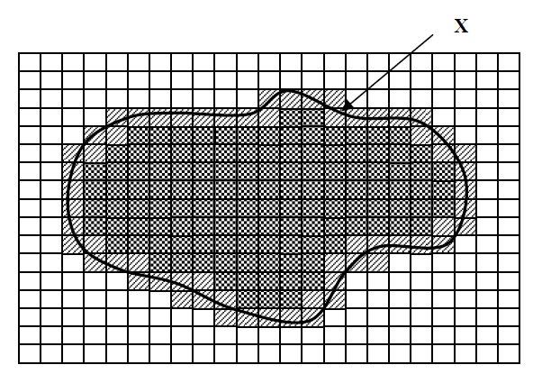
• Lower approximation of the set X includes elements that really belong to the set X.
• Upper approximation of the set X + includes elements that possibly belong to the set X.
• Border (difference between upper and lower approximation) represents an area of ​​indistinguishability.

')

Actually use

Approximate sets are used when working with data tables, which are also called attribute-value tables, or information systems, or decision tables (decision tables). The decision table (decision table) is a triple Τ = (U, C, D), where
U is a set of objects
C is a set of condition attributes,
D is the set of decision attributes.

Sample table

U	C		D
	Headache	Temperature	Flu
U 1	Yes	normal	not
U 2	Yes	high	Yes
U 3	Yes	normal	not
U 4	Yes	very high	not
U 5	not	high	not
U 6	not	very high	Yes
U 7	not	high	Yes
U 8	not	very high	Yes

Table analysis

Sets:
U = {U ₁ , U ₂ , U ₃ , U ₄ , U ₅ , U ₆ , U ₇ , U ₈ }
C = {Headache, Temperature}
D = {Flu}

Possible attribute values:
V _Headache = {yes, no}
V _Temperature = {normal, high, very high}
V _Flu = {yes, no}

The splitting of the set U in accordance with the values ​​of the attribute Headache has the form:

• S _yes = {1, 2, 3, 4}
• S _no = {5, 6, 7, 8}
• S = {{1, 2, 3, 4}, {5, 6, 7, 8}}

The splitting of the set U in accordance with the values ​​of the attribute Temperature has the form:

• S _normal = {1, 3}
• S _high = {2, 5, 7}
• S _{very high} = {4, 6}
• S = {{1, 3}, {2, 5, 7}, {4, 6}}

The partition of the set U in accordance with the values ​​of the attribute of the solution. Influenza is:

• S _yes = {2, 6, 7, 8}
• S _no = {1, 3, 4, 5}
• S = {{2, 6, 7, 8}, {1, 3, 4, 5}}

The data presented in this table, for example, U ₅ and U ₇ are inconsistent, and U ₆ and U ₈ are repeated.

U 5	not	high	not
U 6	not	very high	Yes
U 7	not	high	Yes
U 8	not	very high	Yes

Actually using approximate sets we can “extract” from inaccurate, contradictory data those that are “useful to us”.

What are we going to work on?

The following posts will demonstrate the practical implementation (in Python) of data analysis using this theory, including:

• Algorithm of decision making, consisting of decision rules of the type “IF ... THAT ...”
• Algorithm LEM, LEM2 [Grzymała-Busse, 1992] of generating decision rules like "IF ... THAT ..."