Restore defocused and blurred images
Recovering distorted images is one of the most interesting and important problems in image processing tasks - both from theoretical and practical points of view. Special cases are blurring due to improper focus and blurring - these defects, with which each of you is well acquainted, are very difficult to correct - they were chosen as the topic of the article. With the rest of the distortions (noise, irregular exposure, distortion), mankind has learned how to effectively deal, there are appropriate tools in every self-respecting photo editor.
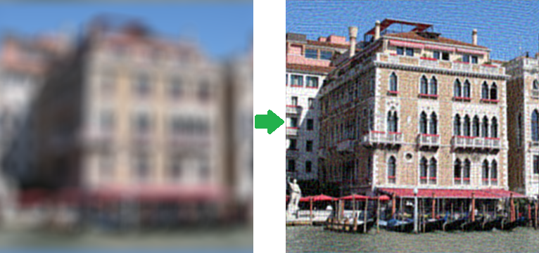
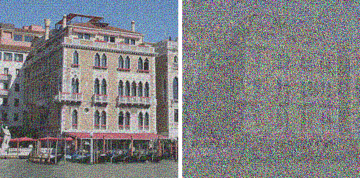
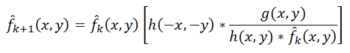
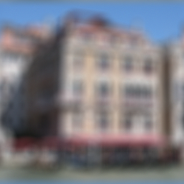
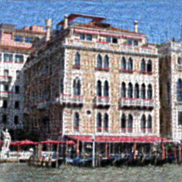
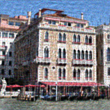
Why is there practically nothing to eliminate blurring and defocusing (unsharp mask doesn’t count) - can this be impossible in principle? In fact, it is possible - the corresponding mathematical apparatus began to be developed about 70 years ago, but, like for many other image processing algorithms, all this has found wide application only in recent times. Here, as a demonstration of the wow effect, a couple of pictures:
')
I did not use the tortured Lena , but found my photo of Venice. The right image is honestly obtained from the left, and without the use of tricks such as 48-bit format (in this case there will be a 100% recovery of the original image) - on the left is the most common PNG, blurred artificially. The result is impressive ... but in practice, not everything is so simple. Under the cat a detailed review of the theory and practical results.
Be careful, lots of pictures in PNG format!
Let's start from afar. Many people think that blurring is an irreversible operation and information is irretrievably lost, because each pixel turns into a spot, everything mixes, and with a large blur radius, we get a uniform color throughout the image. This is not entirely true - all information is simply redistributed according to some law and can be unequivocally restored with some reservations. The only exception is the edges of the image width to the blur radius - there is no full restoration.
Let us demonstrate this “on the fingers” using a small example for a one-dimensional case — imagine that we have a row of pixels with values:
x 1 | x 2 | x 3 | x 4 ... - Original Image
After distortion, the value of each pixel is summed with the value of the left one, i.e. x ' i = x i + x i-1 . In theory, we must also divide by 2, but omit it for simplicity. As a result, we have blurred images with pixel values:
x 1 + x 0 | x 2 + x 1 | x 3 + x 2 | x 4 + x 3 ... - Blurred Image
Now we will try to restore, subtract sequentially the value chain by the scheme - from the second pixel the first, from the third result of the second, from the fourth result of the third and so on, we get:
x 1 + x 0 | x 2 - x 0 | x 3 + x 0 | x 4 - x 0 ... - Refurbished image
As a result, instead of a blurred image, an original image was obtained, to the pixels of which an unknown constant x 0 with an alternating sign was added. This is already much better - this constant can be chosen visually, it can be assumed that it is approximately equal to the value of x 1 , you can automatically choose with such a criterion that the values of the neighboring pixels “jump” as little as possible, etc. But everything changes as soon as we add noise (which is always present in real images). With the scheme described at each step, the noise contribution to the common component will accumulate, which may ultimately give an absolutely unacceptable result, but, as we have seen, the recovery is quite realistic even in such a primitive way.
We now turn to a more formal and scientific description of these processes of distortion and restoration. We will consider only halftone black-and-white images under the assumption that to process a full-color image, it is enough to repeat all the necessary steps for each of the RGB color channels. We introduce the following notation:
f (x, y) - the original undistorted image
h (x, y) is a distorting function
n (x, y) - additive noise
g (x, y) is the result of the distortion, i.e. what we see as a result (blurred or defocused image)
We formulate a distortion process model as follows:
g (x, y) = h (x, y) * f (x, y) + n (x, y) (1)
The task of recovering a distorted image is to find the best approximation f '(x, y) of the original image. Consider each component in more detail. With f (x, y) and g (x, y), everything is quite clear. But about the function h (x, y ) you need to say a few words - what does it look like? In the process of distortion, each pixel of the original image turns into a spot for the case of defocusing and a segment for the case of a simple blurring. Or it can be said on the contrary that each pixel of a distorted image is “assembled” from the pixels of some neighborhood of the original image. All this is superimposed on each other and as a result we get a distorted image. That, according to what law one pixel is smeared or assembled and is called the distortion function. Other synonyms are PSF (Point spread function, i.e. point distribution function), the core of the distorting operator, kernel, and others. The dimension of this function is usually less than the dimension of the image itself - for example, in the initial consideration of the example “on fingers”, the dimension of the function was 2, since each pixel consisted of two.
Let's see how typical distorting functions look like. Hereinafter we will use the tool that has already become standard for such purposes - Matlab, it contains everything necessary for a wide variety of experiments with image processing (and not only) and allows you to focus on the algorithms themselves, shifting all routine work to the library of functions. However, for this you have to pay performance. So back to the PSF, here are some examples of their type:
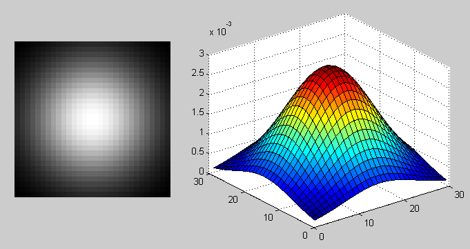
PSF in the case of a Gaussian blur with the fspecial function ('gaussian', 30, 8);
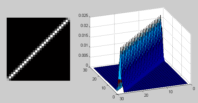
PSF in the case of smearing with fspecial ('motion', 40, 45);
The operation of applying a distorting function to another function (to the image, in this case) is called convolution, i.e. A certain area of the original image is collapsed into one pixel of the distorted image. It is denoted by the operator "*", not to be confused with ordinary multiplication! Mathematically, for an image f with dimensions M x N and a distorting function h with dimensions mxn, this is written as:
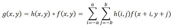 (2)
(2)
Where a = (m - 1) / 2, b = (n - 1) / 2 . The operation inverse to convolution is called deconvolution, and the solution of such a problem is very nontrivial.
It remains to consider the last term responsible for noise, n (x, y) in formula (1). The causes of noise in digital sensors can be very different, but the main ones are thermal oscillations and dark currents. The amount of noise is also influenced by a number of factors, such as ISO value, matrix type, pixel size, temperature, electromagnetic pickups, etc. In most cases, the noise is Gaussian (which is defined by two parameters — average and dispersion), and is also additive, does not correlate with the image and does not depend on pixel coordinates. The last three assumptions are very important for further work.
We now return to the original formulation of the restoration problem — we need to somehow invert the convolution, while not forgetting the noise. It is clear from formula (2) that getting f (x, y) from g (x, y) is not so easy - if you solve what is called head-on, you get a huge system of equations. But the Fourier transform comes to help us; we will not dwell on it in detail; quite a lot has already been said on this topic. So, there is a convolution theorem, which states that the convolution operation in the spatial domain is equivalent to the usual multiplication in the frequency domain (and the multiplication is element-wise, not matrix). Accordingly, the inverse convolution operation is equivalent to division in the frequency domain, i.e. this can be written as:
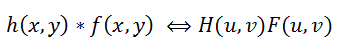 (3)
(3)
Where H (u, v), F (u, v) are the Fourier transforms of the corresponding functions. So the process of distortion from the formula (1) can be rewritten in the frequency domain as:
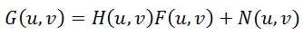 (four)
Here it is suggested to divide this equality by H (u, v) and get the following estimate F ^ (u, v) of the original image:
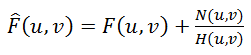 (five)
This is called inverse filtering, but in practice it almost never works. Why so? To answer this question, we look at the last term in formula (5) - if the function H (u, v) takes a value close to zero or zero, then the contribution of this term will be dominant. This is almost always found in real-world examples — to explain this, let us recall how the spectrum looks after the Fourier transform.
Take the original image
transform it into a halftone and, using Matlab, we obtain the spectrum:
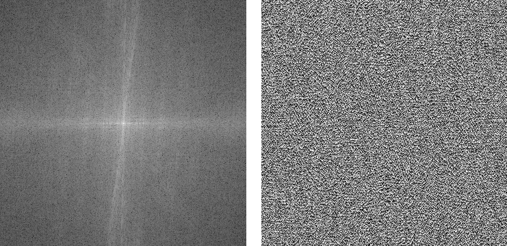
As a result, we obtain two components: amplitude and phase spectra. By the way, many people forget about the phase. Note that the amplitude spectrum is shown in a logarithmic scale, since its values vary very much - by several orders of magnitude; in the center, the maximum values (of the order of millions) and rapidly decrease to almost zero as the distance from the center increases. It is because of this that the inverse filtering will work only at zero or almost zero noise values. Let's demonstrate this in practice using the following script:
It is clearly seen that the addition of even very small noise leads to significant interference, which greatly limits the practical application of the method.
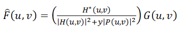
But there are approaches that take into account the presence of noise in the image - one of the most famous and the very first is the Wiener filter. He considers the image and noise as random processes and finds such an estimate f ′ for the undistorted image f , so that the standard deviation of these values is minimal. The minimum of this deviation is achieved on the function in the frequency domain:
 (6)
(6)
This result was obtained by Wiener in 1942. We will not give a detailed conclusion here, those who are interested can see it here . The function S here denotes the energy spectra of the noise and the original image, respectively - since these quantities are rarely known, the fraction S n / S f is replaced by some constant K, which can be approximately characterized as a signal-to-noise ratio.
The next method is “smoothing least squares filtering with a connection”, other names: “Tikhonov filtering”, “Tikhonov regularization”. His idea is to formulate the problem in a matrix form with further solution of the corresponding optimization problem. This solution is written as:
 (7)
(7)
Where y is the regularization parameter, and P (u, v) is the Fourier transform of the Laplace operator (3 * 3 matrix).
Another interesting approach was proposed independently by Richard [Richardson, 1972] and Lucy [Lucy, 1974]. The method is called the "Lucy-Richardson method." Its distinguishing feature is that it is non-linear, unlike the first three - which can potentially give better results. The second peculiarity - the method is iterative; accordingly, difficulties arise with the criterion for stopping iterations. The basic idea is to use the maximum likelihood method for which it is assumed that the image obeys the Poisson distribution. The formulas for the calculation are quite simple, without using the Fourier transform - everything is done in the spatial domain:
 (eight)
Here the symbol "*", as before, denotes the operation of convolution. This method is widely used in programs for processing astronomical photographs - in them the use of deconvolution (instead of an unsharp mask, as in photo editors) is a de facto standard. As an example, Astra Image, here are examples of deconvolution . The computational complexity of the method is very large - processing of a medium photo, depending on the number of iterations, can be known for many hours and even days.
The last considered method, or rather, a whole family of methods that are now being actively developed and developed, is blind deconvolution. In all previous methods it was assumed that the distorting function of the PSF is precisely known, in reality it is not so, usually the PSF is known only approximately by the nature of the visible distortion. Blind deconvolution is an attempt to take this into account. The principle is quite simple, if you don’t go into details - the first approximation of PSF is selected, then deconvolution is done using one of the methods, after which some criterion determines the degree of quality, based on it the PSF function is refined and the iteration is repeated until the desired result is achieved.
Now, with the theory of everything - let's move on to practice, let's start by comparing the listed methods on the image with artificial blurring and noise.
Results:
Wiener Filter
Regularization Tikhonov
Lucy-richardson filter
Blind deconvolution
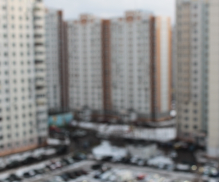
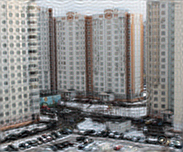
And at the end of the first part we will touch upon examples of real images. Before that, all the distortions were artificial, which is certainly good for running in and studying, but it is very interesting to see how all this will work with real photos. Here is one example of such an image taken with a Canon 500D DSLR camera with manual focus focus:
Next, run a simple script:
And we get the following result:
As you can see, new details have appeared on the image, clarity has become much higher, although noise also appeared in the form of “ringing” on contrasting borders.
And an example with a real lubricant - for its implementation, the camera was mounted on a tripod, a relatively long exposure was set and a uniform motion was obtained at the moment of shutter release:
The script is about the same, only the type of PSF is now “motion”:
Result:
The quality, again, has improved markedly - the frames on the windows and cars have become visible. Artifacts are already different than in the previous defocusing example.
At this interesting and finish the first part.
In the second part, I will focus on the problems of processing real images - building PSF and evaluating them, consider more complex and advanced deconvolution techniques, methods for eliminating ring type defects, review and compare existing software, and so on.
PS Not so long ago an article was published on the Habré about Fixing blurry photos in a new version of Photoshop
For those who want to play around with a similar technology to remove blurring (perhaps the one that will be used in Photoshop), you can download the demo version of the application, see recovery examples, and read about the principle of operation .
Gonzalez R., Woods R. Digital Image Processing
Gonzalez R., Woods R., Eddins S. Digital Image Processing in MATLAB
UPD: Continuation Link
Why is there practically nothing to eliminate blurring and defocusing (unsharp mask doesn’t count) - can this be impossible in principle? In fact, it is possible - the corresponding mathematical apparatus began to be developed about 70 years ago, but, like for many other image processing algorithms, all this has found wide application only in recent times. Here, as a demonstration of the wow effect, a couple of pictures:
')
I did not use the tortured Lena , but found my photo of Venice. The right image is honestly obtained from the left, and without the use of tricks such as 48-bit format (in this case there will be a 100% recovery of the original image) - on the left is the most common PNG, blurred artificially. The result is impressive ... but in practice, not everything is so simple. Under the cat a detailed review of the theory and practical results.
Be careful, lots of pictures in PNG format!
Introduction
Let's start from afar. Many people think that blurring is an irreversible operation and information is irretrievably lost, because each pixel turns into a spot, everything mixes, and with a large blur radius, we get a uniform color throughout the image. This is not entirely true - all information is simply redistributed according to some law and can be unequivocally restored with some reservations. The only exception is the edges of the image width to the blur radius - there is no full restoration.
Let us demonstrate this “on the fingers” using a small example for a one-dimensional case — imagine that we have a row of pixels with values:
x 1 | x 2 | x 3 | x 4 ... - Original Image
After distortion, the value of each pixel is summed with the value of the left one, i.e. x ' i = x i + x i-1 . In theory, we must also divide by 2, but omit it for simplicity. As a result, we have blurred images with pixel values:
x 1 + x 0 | x 2 + x 1 | x 3 + x 2 | x 4 + x 3 ... - Blurred Image
Now we will try to restore, subtract sequentially the value chain by the scheme - from the second pixel the first, from the third result of the second, from the fourth result of the third and so on, we get:
x 1 + x 0 | x 2 - x 0 | x 3 + x 0 | x 4 - x 0 ... - Refurbished image
As a result, instead of a blurred image, an original image was obtained, to the pixels of which an unknown constant x 0 with an alternating sign was added. This is already much better - this constant can be chosen visually, it can be assumed that it is approximately equal to the value of x 1 , you can automatically choose with such a criterion that the values of the neighboring pixels “jump” as little as possible, etc. But everything changes as soon as we add noise (which is always present in real images). With the scheme described at each step, the noise contribution to the common component will accumulate, which may ultimately give an absolutely unacceptable result, but, as we have seen, the recovery is quite realistic even in such a primitive way.
Distortion process model
We now turn to a more formal and scientific description of these processes of distortion and restoration. We will consider only halftone black-and-white images under the assumption that to process a full-color image, it is enough to repeat all the necessary steps for each of the RGB color channels. We introduce the following notation:
f (x, y) - the original undistorted image
h (x, y) is a distorting function
n (x, y) - additive noise
g (x, y) is the result of the distortion, i.e. what we see as a result (blurred or defocused image)
We formulate a distortion process model as follows:
g (x, y) = h (x, y) * f (x, y) + n (x, y) (1)
The task of recovering a distorted image is to find the best approximation f '(x, y) of the original image. Consider each component in more detail. With f (x, y) and g (x, y), everything is quite clear. But about the function h (x, y ) you need to say a few words - what does it look like? In the process of distortion, each pixel of the original image turns into a spot for the case of defocusing and a segment for the case of a simple blurring. Or it can be said on the contrary that each pixel of a distorted image is “assembled” from the pixels of some neighborhood of the original image. All this is superimposed on each other and as a result we get a distorted image. That, according to what law one pixel is smeared or assembled and is called the distortion function. Other synonyms are PSF (Point spread function, i.e. point distribution function), the core of the distorting operator, kernel, and others. The dimension of this function is usually less than the dimension of the image itself - for example, in the initial consideration of the example “on fingers”, the dimension of the function was 2, since each pixel consisted of two.
Distorting functions
Let's see how typical distorting functions look like. Hereinafter we will use the tool that has already become standard for such purposes - Matlab, it contains everything necessary for a wide variety of experiments with image processing (and not only) and allows you to focus on the algorithms themselves, shifting all routine work to the library of functions. However, for this you have to pay performance. So back to the PSF, here are some examples of their type:
PSF in the case of a Gaussian blur with the fspecial function ('gaussian', 30, 8);
PSF in the case of smearing with fspecial ('motion', 40, 45);
The operation of applying a distorting function to another function (to the image, in this case) is called convolution, i.e. A certain area of the original image is collapsed into one pixel of the distorted image. It is denoted by the operator "*", not to be confused with ordinary multiplication! Mathematically, for an image f with dimensions M x N and a distorting function h with dimensions mxn, this is written as:
(2)Where a = (m - 1) / 2, b = (n - 1) / 2 . The operation inverse to convolution is called deconvolution, and the solution of such a problem is very nontrivial.
Noise model
It remains to consider the last term responsible for noise, n (x, y) in formula (1). The causes of noise in digital sensors can be very different, but the main ones are thermal oscillations and dark currents. The amount of noise is also influenced by a number of factors, such as ISO value, matrix type, pixel size, temperature, electromagnetic pickups, etc. In most cases, the noise is Gaussian (which is defined by two parameters — average and dispersion), and is also additive, does not correlate with the image and does not depend on pixel coordinates. The last three assumptions are very important for further work.
Convolution theorem
We now return to the original formulation of the restoration problem — we need to somehow invert the convolution, while not forgetting the noise. It is clear from formula (2) that getting f (x, y) from g (x, y) is not so easy - if you solve what is called head-on, you get a huge system of equations. But the Fourier transform comes to help us; we will not dwell on it in detail; quite a lot has already been said on this topic. So, there is a convolution theorem, which states that the convolution operation in the spatial domain is equivalent to the usual multiplication in the frequency domain (and the multiplication is element-wise, not matrix). Accordingly, the inverse convolution operation is equivalent to division in the frequency domain, i.e. this can be written as:
(3)Where H (u, v), F (u, v) are the Fourier transforms of the corresponding functions. So the process of distortion from the formula (1) can be rewritten in the frequency domain as:
(four)Inverse filtering
Here it is suggested to divide this equality by H (u, v) and get the following estimate F ^ (u, v) of the original image:
(five)This is called inverse filtering, but in practice it almost never works. Why so? To answer this question, we look at the last term in formula (5) - if the function H (u, v) takes a value close to zero or zero, then the contribution of this term will be dominant. This is almost always found in real-world examples — to explain this, let us recall how the spectrum looks after the Fourier transform.
Take the original image
transform it into a halftone and, using Matlab, we obtain the spectrum:
% Load image I = imread('image_src.png'); figure(1); imshow(I); title(' '); % Convert image into grayscale I = rgb2gray(I); % Compute Fourier Transform and center it fftRes = fftshift(fft2(I)); % Show result figure(2); imshow(mat2gray(log(1+abs(fftRes)))); title('FFT - ( )'); figure(3); imshow(mat2gray(angle(fftRes))); title('FFT - '); As a result, we obtain two components: amplitude and phase spectra. By the way, many people forget about the phase. Note that the amplitude spectrum is shown in a logarithmic scale, since its values vary very much - by several orders of magnitude; in the center, the maximum values (of the order of millions) and rapidly decrease to almost zero as the distance from the center increases. It is because of this that the inverse filtering will work only at zero or almost zero noise values. Let's demonstrate this in practice using the following script:
% Load image I = im2double(imread('image_src.png')); figure(1); imshow(I); title(' '); % Blur image Blurred = imfilter(I, PSF,'circular','conv' ); figure(2); imshow(Blurred); title(' '); % Add noise noise_mean = 0; noise_var = 0.0; Blurred = imnoise(Blurred, 'gaussian', noise_mean, noise_var); % Deconvolution figure(3); imshow(deconvwnr(Blurred, PSF, 0)); title(''); noise_var = 0.0000001 noise_var = 0.000005
It is clearly seen that the addition of even very small noise leads to significant interference, which greatly limits the practical application of the method.
Existing approaches for deconvolution
But there are approaches that take into account the presence of noise in the image - one of the most famous and the very first is the Wiener filter. He considers the image and noise as random processes and finds such an estimate f ′ for the undistorted image f , so that the standard deviation of these values is minimal. The minimum of this deviation is achieved on the function in the frequency domain:
(6)This result was obtained by Wiener in 1942. We will not give a detailed conclusion here, those who are interested can see it here . The function S here denotes the energy spectra of the noise and the original image, respectively - since these quantities are rarely known, the fraction S n / S f is replaced by some constant K, which can be approximately characterized as a signal-to-noise ratio.
The next method is “smoothing least squares filtering with a connection”, other names: “Tikhonov filtering”, “Tikhonov regularization”. His idea is to formulate the problem in a matrix form with further solution of the corresponding optimization problem. This solution is written as:
(7)Where y is the regularization parameter, and P (u, v) is the Fourier transform of the Laplace operator (3 * 3 matrix).
Another interesting approach was proposed independently by Richard [Richardson, 1972] and Lucy [Lucy, 1974]. The method is called the "Lucy-Richardson method." Its distinguishing feature is that it is non-linear, unlike the first three - which can potentially give better results. The second peculiarity - the method is iterative; accordingly, difficulties arise with the criterion for stopping iterations. The basic idea is to use the maximum likelihood method for which it is assumed that the image obeys the Poisson distribution. The formulas for the calculation are quite simple, without using the Fourier transform - everything is done in the spatial domain:
(eight)Here the symbol "*", as before, denotes the operation of convolution. This method is widely used in programs for processing astronomical photographs - in them the use of deconvolution (instead of an unsharp mask, as in photo editors) is a de facto standard. As an example, Astra Image, here are examples of deconvolution . The computational complexity of the method is very large - processing of a medium photo, depending on the number of iterations, can be known for many hours and even days.
The last considered method, or rather, a whole family of methods that are now being actively developed and developed, is blind deconvolution. In all previous methods it was assumed that the distorting function of the PSF is precisely known, in reality it is not so, usually the PSF is known only approximately by the nature of the visible distortion. Blind deconvolution is an attempt to take this into account. The principle is quite simple, if you don’t go into details - the first approximation of PSF is selected, then deconvolution is done using one of the methods, after which some criterion determines the degree of quality, based on it the PSF function is refined and the iteration is repeated until the desired result is achieved.
Practice
Now, with the theory of everything - let's move on to practice, let's start by comparing the listed methods on the image with artificial blurring and noise.
% Load image I = im2double(imread('image_src.png')); figure(1); imshow(I); title(' '); % Blur image PSF = fspecial('disk', 15); Blurred = imfilter(I, PSF,'circular','conv' ); % Add noise noise_mean = 0; noise_var = 0.00001; Blurred = imnoise(Blurred, 'gaussian', noise_mean, noise_var); figure(2); imshow(Blurred); title(' '); estimated_nsr = noise_var / var(Blurred(:)); % Restore image figure(3), imshow(deconvwnr(Blurred, PSF, estimated_nsr)), title('Wiener'); figure(4); imshow(deconvreg(Blurred, PSF)); title('Regul'); figure(5); imshow(deconvblind(Blurred, PSF, 100)); title('Blind'); figure(6); imshow(deconvlucy(Blurred, PSF, 100)); title('Lucy'); Results:
Wiener Filter
Regularization Tikhonov
Lucy-richardson filter
Blind deconvolution
Conclusion
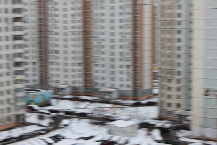
And at the end of the first part we will touch upon examples of real images. Before that, all the distortions were artificial, which is certainly good for running in and studying, but it is very interesting to see how all this will work with real photos. Here is one example of such an image taken with a Canon 500D DSLR camera with manual focus focus:
Next, run a simple script:
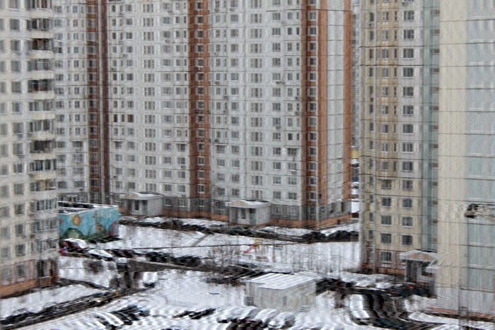
% Load image I = im2double(imread('IMG_REAL.PNG')); figure(1); imshow(I); title(' '); %PSF PSF = fspecial('disk', 8); noise_mean = 0; noise_var = 0.0001; estimated_nsr = noise_var / var(I(:)); I = edgetaper(I, PSF); figure(2); imshow(deconvwnr(I, PSF, estimated_nsr)); title(''); And we get the following result:
As you can see, new details have appeared on the image, clarity has become much higher, although noise also appeared in the form of “ringing” on contrasting borders.
And an example with a real lubricant - for its implementation, the camera was mounted on a tripod, a relatively long exposure was set and a uniform motion was obtained at the moment of shutter release:
The script is about the same, only the type of PSF is now “motion”:
% Load image I = im2double(imread('IMG_REAL_motion_blur.PNG')); figure(1); imshow(I); title(' '); %PSF PSF = fspecial('motion', 14, 0); noise_mean = 0; noise_var = 0.0001; estimated_nsr = noise_var / var(I(:)); I = edgetaper(I, PSF); figure(2); imshow(deconvwnr(I, PSF, estimated_nsr)); title(''); Result:
The quality, again, has improved markedly - the frames on the windows and cars have become visible. Artifacts are already different than in the previous defocusing example.
At this interesting and finish the first part.
In the second part, I will focus on the problems of processing real images - building PSF and evaluating them, consider more complex and advanced deconvolution techniques, methods for eliminating ring type defects, review and compare existing software, and so on.
PS Not so long ago an article was published on the Habré about Fixing blurry photos in a new version of Photoshop
For those who want to play around with a similar technology to remove blurring (perhaps the one that will be used in Photoshop), you can download the demo version of the application, see recovery examples, and read about the principle of operation .
Literature
Gonzalez R., Woods R. Digital Image Processing
Gonzalez R., Woods R., Eddins S. Digital Image Processing in MATLAB
UPD: Continuation Link
-Vladimir Yuzhikov
Source: https://habr.com/ru/post/136853/
All Articles