Neural network in scheme
Since the topic of neural networks has recently been raised again, I decided to show a small implementation of the National Assembly, which is being taught by the back propagation method of error, written in a scheme. At the same time I will tell you in detail how this all works, for beginners of the genre. Only the simplest type of networks will be considered, without looping and skipping layers.

Let's start with a description of the biological component. If we omit the details, the neuron is a complex cell with several entrances - dendrites and one output - an axon. At the inputs of the neuron periodically receive electrical signals from the senses or other neurons. The input signals are summed, and with their sufficient strength, the neuron outputs its electrical signal to the axon, where it is received by the dendrite of another neuron, or an internal organ. If the signal level is too low, the neuron is silent. Having the structure of a sufficient number of such neurons, it is possible to solve quite complex tasks.
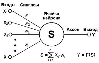
An artificial neural network is a graph whose vertices are equivalent to neurons, and the edges are axons / dendrites, the connection of which is called synapses. Each artificial neuron consists of several synapses, with its own gain or signal attenuation, activation function, pass value and output axon. The signal at the input of each synapse is multiplied by its coefficient (connection weight), after which the signals are summed and transmitted, as an argument, to the activation function, which transmits it to the axon, where it is received by other neurons.
')
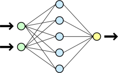
Neurons are grouped by layers. Each neuron of one layer is connected with all neurons of the next layer, as with all neurons of the previous layer, but not connected with other neurons of its layer. The neural network itself consists of at least two layers of neurons - the input layer and the output layer, between which there can be an arbitrary number of so-called hidden layers. The signal propagates only in one direction - from the input layer to the output one. It is worth noting here that there are other types of networks in which signal propagation occurs differently.
Someone may have a question - why all this? In fact, the neural network makes it possible to solve problems that are difficult to describe using standard algorithms. One of the typical purposes is image recognition. By “showing” the neural network a certain picture and indicating what output pattern should be in the case of this picture, we are teaching the NA. If you demonstrate the network a sufficient number of different options for entry, the network learn to look for something in common between the patterns and use it to recognize images that she has never seen before. It should be noted that the ability to recognize images depends on the structure of the network, as well as on the sample of images used for training.
We now turn directly to the implementation. The language Scheme was used, which IMHO is the most beautiful and concise dialect of LISP. The implementation was written in MIT-Scheme, but should work without any problems on other interpreters.
The implementation uses the following types of lists:
(n lst) - neuron. neuron, instead of lst contains a list with synaptic signal amplification factors. For example: (n (1 2 4)).
(l lst) - layer. layer consisting of neurons. Instead of lst contains a list of neurons. An example of a layer of 2 neurons (l ((n (0.1 0.6 0.2)) (n (0.8 0.4 0.4))))
(lst) - the usual list, without any symbol at the beginning of the list - the usual neural network. Instead of lst contains a list of layers. For example:
((l ((n (0.1 0.6 0.2)) (n (0.5 0.1 0.7)) (n (0.8 0.4 0.4))))
(l ((n (0.3 0.8 0.9)) (n (0.4 0.9 0.1))) (n (0.9 0.9 0.9)))))
Some abbreviations are used in the code:
; out - neuron output - neuron output
; wh - weight - weight of the connection
; res - result - the result of calculating the entire neuron layer
; akt - activation - the result of neuron activation
; n - neuron
; l - layer
; net - network
; mk - make
; proc - process
Let's start by creating a neuron, which is boring and not interesting:
Let's proceed to layer creation:
input - the number of inputs in the neurons of this layer
n is the number of neurons in the layer.
lst - a list of ready-made neurons.
Knowing the number of inputs, we order so many random numbers from lst-rand, pack them with n-mk and put them in lst1. Check whether you need more neurons, if it was not the last neuron, then reduce the counter and repeat the operation. If this is the last neuron, we pack them with l-mk.
Next we will create the network itself. This is done using the function net-make. Lay - a list with the number of neurons for each layer. The first number is the list of entries for the first layer.
The function is syntactic sugar and is made to simplify the call. In fact, net-make-new will be called, which simply has a separate parameter for the number of inputs on the first layer. The function l-mk-new is called recursively to create layers and add them to lst1.
Now we have a newly created network. Let's take a function to use it. The activation function was selected:
For those who are not used to Lisp syntax, this is just x / (| x | + p), where the p parameter makes the function graph sharper or smoother.
neuron - contains an activated neuron,
input - the values of the inputs of synapses.
In response, we obtain the output of the neuron axon. 4 - parameter for the activation function, was selected by experiments. You can safely change to any other. Now let's do the activation of the whole layer.
input - the outputs of the neurons of the previous layer,
l - the layer itself
n-inp-lst - returns a list of neurons of this layer.
We will rise to a higher level and make the activation function of the entire network.
net - the network itself,
input - data submitted to the inputs of the first layer.
Input is used to process the first layer, later we use the output of the previous layer as the input of the next one. If the layer is the last - its result is displayed as the result of the entire network.
With the creation and processing of the network sort of sorted out. We now turn to the more interesting part - learning. Here we go from the top down. Those. from network level to lower levels. The network learning function is net-study.
where net is the network itself,
lst - list of examples
spd - learning speed.
net-check-lst - checks the correctness of network responses for examples from lst
net-study-lst - produces network training
The speed of learning is the step of changing the weights of each neuron. Very complex parameter, since with a small step, you can wait a long time for the results of training, and with a large step, you can constantly skip the desired interval. net-study is performed until net-check-lst is passed.
Here added l-check. At the moment they are not doing anything, but at the testing stage they were catching the transmitted values using it.
Net-study2 compares the maximum exit number in the pattern with the maximum output number after the fact. If they match, we return the trained network; if not, we continue the training.
wh - list of incoming weights of all neurons of the network
out - contains a list of outputs of all neurons in the network
err - list with errors for each neuron
Net-spd * err - multiplies the speed with a list of errors by the weights of the neuron.
Net-err + wh - adds the calculated error to the list of weights.
Net-make-data makes a new network from the received data.
Well, now the most interesting - counting errors. To change the weights, the function will be used:

Where
Wij is the weight from neuron i to neuron j,
Xi is the output of neuron i,
R - learning step,
Gj - error value for neuron j.
When calculating the error for the output layer, the function is used:

Where
Dj - the desired output of the neuron j,
Yj - the current output of the neuron j.
For all previous layers, the function is used:

where k runs all the neurons of the layer with the number one greater than that of the one that owns the neuron j.
Now a little about what is happening:
Wh-lst - contains the values of the connections of each neuron, with the next layer,
Err-lst - contains an error for the output network layer, in the future we fill it with errors of other layers,
Out-lst - the value of the output of each neuron
Recursively process these three lists, according to the function.
Now, strictly speaking, how it all works. The example will be simple, but if you wish, you can recognize more complex things. We will have only four simple patterns for the letters T, O, I, U. We declare their display:
(define t '(
1 1 1
0 1 0
0 1 0))
(define o '(
1 1 1
1 0 1
1 1 1))
(define i '(
0 1 0
0 1 0
0 1 0))
(define u '(
1 0 1
1 0 1
1 1 1))
Now we will create a form for learning. Each letter corresponds to one of 4 exits.
(define letters (list
(list o '(1 0 0 0))
(list t '(0 1 0 0))
(list i '(0 0 1 0))
(list u '(0 0 0 1))))
Now we will create a new network that has 9 inputs, 3 layers and 4 outputs.
(define test (net-make '(9 8 4)))
We will train the network using our example. Letters - a list of examples. 0.5 - learning step.
(define test1 (net-study test letters 0.5))
As a result, we have the test1 network, which recognizes our patterns. Test it:
(net-proc test1 o)
> (.3635487227069449 .32468771459315143 .20836372502023912 .3635026264793502)
To make it a little clearer, you can do this:
(net-proc-num test1 o)
> 0
Those. the largest output was zero output. Same for other patterns:
(net-proc-num test1 i)
> 2
We can slightly damage the image and check whether it will be recognized:
(net-proc-num test1
'(
0 1 0
1 0 1
0 1 0))
> 0
(net-proc-num test1
'(
0 0 1
0 1 0
0 1 0))
> 1
Even a damaged image is completely different. True, a controversial situation can be made, for example, in such a case, the network will confuse the pattern T with the pattern I. The outputs will be very close.
(net-proc test1
'(
0 1 1
0 1 0
0 0 0))
> (.17387815810580473 .2731127800467817 .31253464734295566 -6.323399331678244e-3)
As you can see, the network offers 1 and 2 outputs. Those. The patterns are quite similar and the network considers 2 patterns more likely.
PS I assume that all this is all too messy, but maybe someone will find it interesting.
PSS A separate request for LISP-ers. This is the first time I publicly post my scheme code, so I will be grateful for the criticism.
Sources:
1. oasis.peterlink.ru/~dap/nneng/nnlinks/nbdoc/bp_task.htm#learn - for functions and inspiration
2. ru.wikipedia.org/wiki/Artificial_Neuron_Network - hence the picture and some information is fooled
3. alife.narod.ru/lectures/neural/Neu_ch03.htm - from here took the picture
4. iklub.rf / neur-1.html
Full source on pastbin:
pastebin.com/erer2BnQ
Let's start with a description of the biological component. If we omit the details, the neuron is a complex cell with several entrances - dendrites and one output - an axon. At the inputs of the neuron periodically receive electrical signals from the senses or other neurons. The input signals are summed, and with their sufficient strength, the neuron outputs its electrical signal to the axon, where it is received by the dendrite of another neuron, or an internal organ. If the signal level is too low, the neuron is silent. Having the structure of a sufficient number of such neurons, it is possible to solve quite complex tasks.
An artificial neural network is a graph whose vertices are equivalent to neurons, and the edges are axons / dendrites, the connection of which is called synapses. Each artificial neuron consists of several synapses, with its own gain or signal attenuation, activation function, pass value and output axon. The signal at the input of each synapse is multiplied by its coefficient (connection weight), after which the signals are summed and transmitted, as an argument, to the activation function, which transmits it to the axon, where it is received by other neurons.
')
Neurons are grouped by layers. Each neuron of one layer is connected with all neurons of the next layer, as with all neurons of the previous layer, but not connected with other neurons of its layer. The neural network itself consists of at least two layers of neurons - the input layer and the output layer, between which there can be an arbitrary number of so-called hidden layers. The signal propagates only in one direction - from the input layer to the output one. It is worth noting here that there are other types of networks in which signal propagation occurs differently.
Someone may have a question - why all this? In fact, the neural network makes it possible to solve problems that are difficult to describe using standard algorithms. One of the typical purposes is image recognition. By “showing” the neural network a certain picture and indicating what output pattern should be in the case of this picture, we are teaching the NA. If you demonstrate the network a sufficient number of different options for entry, the network learn to look for something in common between the patterns and use it to recognize images that she has never seen before. It should be noted that the ability to recognize images depends on the structure of the network, as well as on the sample of images used for training.
We now turn directly to the implementation. The language Scheme was used, which IMHO is the most beautiful and concise dialect of LISP. The implementation was written in MIT-Scheme, but should work without any problems on other interpreters.
The implementation uses the following types of lists:
(n lst) - neuron. neuron, instead of lst contains a list with synaptic signal amplification factors. For example: (n (1 2 4)).
(l lst) - layer. layer consisting of neurons. Instead of lst contains a list of neurons. An example of a layer of 2 neurons (l ((n (0.1 0.6 0.2)) (n (0.8 0.4 0.4))))
(lst) - the usual list, without any symbol at the beginning of the list - the usual neural network. Instead of lst contains a list of layers. For example:
((l ((n (0.1 0.6 0.2)) (n (0.5 0.1 0.7)) (n (0.8 0.4 0.4))))
(l ((n (0.3 0.8 0.9)) (n (0.4 0.9 0.1))) (n (0.9 0.9 0.9)))))
Some abbreviations are used in the code:
; out - neuron output - neuron output
; wh - weight - weight of the connection
; res - result - the result of calculating the entire neuron layer
; akt - activation - the result of neuron activation
; n - neuron
; l - layer
; net - network
; mk - make
; proc - process
Let's start by creating a neuron, which is boring and not interesting:
(define (n-mk lst) ;make new neuron
(list 'n lst))
Let's proceed to layer creation:
(define (l-mk-new input n lst) ;makes new layer
(let ( (lst1 (append lst (list (n-mk (lst-rand input))))) )
(if (= n 1) (l-mk lst1) (l-mk-new input (- n 1) lst1))))
input - the number of inputs in the neurons of this layer
n is the number of neurons in the layer.
lst - a list of ready-made neurons.
Knowing the number of inputs, we order so many random numbers from lst-rand, pack them with n-mk and put them in lst1. Check whether you need more neurons, if it was not the last neuron, then reduce the counter and repeat the operation. If this is the last neuron, we pack them with l-mk.
Next we will create the network itself. This is done using the function net-make. Lay - a list with the number of neurons for each layer. The first number is the list of entries for the first layer.
(define (net-make lay)
(net-mk-new (car lay) (cdr lay) '()))
The function is syntactic sugar and is made to simplify the call. In fact, net-make-new will be called, which simply has a separate parameter for the number of inputs on the first layer. The function l-mk-new is called recursively to create layers and add them to lst1.
(define (net-mk-new input n-lst lst)
(let ( (lst1 (lst-push-b (l-mk-new input (car n-lst) '()) lst)) )
(if (= (length n-lst) 1) lst1 (net-mk-new (car n-lst) (cdr n-lst) lst1))))
Now we have a newly created network. Let's take a function to use it. The activation function was selected:
(define (n-akt x param) ;neuron activation function
(/ x (+ (abs x) param)))
For those who are not used to Lisp syntax, this is just x / (| x | + p), where the p parameter makes the function graph sharper or smoother.
(define (n-proc neuron input) ;process single neuron
(n-akt (lst-sum (lst-mul (n-inp-lst neuron) input )) 4))
neuron - contains an activated neuron,
input - the values of the inputs of synapses.
In response, we obtain the output of the neuron axon. 4 - parameter for the activation function, was selected by experiments. You can safely change to any other. Now let's do the activation of the whole layer.
(define (l-proc l input) ;proceses a layer
(map (lambda(x)(n-proc x input)) (n-inp-lst l)))
input - the outputs of the neurons of the previous layer,
l - the layer itself
n-inp-lst - returns a list of neurons of this layer.
We will rise to a higher level and make the activation function of the entire network.
(define (net-proc net input)
(let ( (l (l-proc (car net) input)) )
(if (= 1 (length net)) l
(net-proc (cdr net) l))))
net - the network itself,
input - data submitted to the inputs of the first layer.
Input is used to process the first layer, later we use the output of the previous layer as the input of the next one. If the layer is the last - its result is displayed as the result of the entire network.
With the creation and processing of the network sort of sorted out. We now turn to the more interesting part - learning. Here we go from the top down. Those. from network level to lower levels. The network learning function is net-study.
(define (net-study net lst spd) ;studys net for each example from the list smpl ((inp)(out))
(if (net-check-lst net lst) net
(net-study (net-study-lst net lst spd) lst spd)))
where net is the network itself,
lst - list of examples
spd - learning speed.
net-check-lst - checks the correctness of network responses for examples from lst
net-study-lst - produces network training
The speed of learning is the step of changing the weights of each neuron. Very complex parameter, since with a small step, you can wait a long time for the results of training, and with a large step, you can constantly skip the desired interval. net-study is performed until net-check-lst is passed.
(define (net-study-lst net lst spd)
(let ( (x (net-study1 net (caar lst) (cadar lst) spd)) )
(if (= 1 (length lst)) x
(net-study-lst x (cdr lst) spd))))

(define (net-study1 net inp need spd)
(net-study2 net (l-check inp) need spd))
Here added l-check. At the moment they are not doing anything, but at the testing stage they were catching the transmitted values using it.
(define (net-study2 net inp need spd)
(let ( (x (net-study3 net inp need spd)))
(if (= (caar (lst-order-max need))(caar (lst-order-max (net-proc x inp))))
x
(net-study2 x inp need spd))))
Net-study2 compares the maximum exit number in the pattern with the maximum output number after the fact. If they match, we return the trained network; if not, we continue the training.
(define (net-study3 net inp need spd)
(let ((err (net-spd*err spd (slice (net-err net inp need) 1 0)))
(wh (net-inp-wh net))
(out (slice (net-proc-res-out net inp) 0 -1)))
(net-mk-data (net-err+wh wh (map (lambda(xy)(lst-lst-mul xy)) out err)))))
wh - list of incoming weights of all neurons of the network
out - contains a list of outputs of all neurons in the network
err - list with errors for each neuron
Net-spd * err - multiplies the speed with a list of errors by the weights of the neuron.
Net-err + wh - adds the calculated error to the list of weights.
Net-make-data makes a new network from the received data.
Well, now the most interesting - counting errors. To change the weights, the function will be used:
Where
Wij is the weight from neuron i to neuron j,
Xi is the output of neuron i,
R - learning step,
Gj - error value for neuron j.
When calculating the error for the output layer, the function is used:
Where
Dj - the desired output of the neuron j,
Yj - the current output of the neuron j.
For all previous layers, the function is used:
where k runs all the neurons of the layer with the number one greater than that of the one that owns the neuron j.
(define (net-err net inp need) ;networks error list for each neuron
(let ( (wh-lst (reverse (net-out-wh net)))
(err-lst (list (net-out-err net inp need)))
(out-lst (reverse (slice (net-proc-res-out net inp) 0 -1))))
(net-err2 out-lst err-lst wh-lst)))

(define (net-err2 out-lst err-lst wh-lst)
(let ( (err-lst1 (lst-push (l-err (car out-lst) (car err-lst) (first wh-lst)) err-lst)) )
(if (lst-if out-lst wh-lst) err-lst1 (net-err2 (cdr out-lst) err-lst1 (cdr wh-lst)))))
Now a little about what is happening:
Wh-lst - contains the values of the connections of each neuron, with the next layer,
Err-lst - contains an error for the output network layer, in the future we fill it with errors of other layers,
Out-lst - the value of the output of each neuron
Recursively process these three lists, according to the function.
Now, strictly speaking, how it all works. The example will be simple, but if you wish, you can recognize more complex things. We will have only four simple patterns for the letters T, O, I, U. We declare their display:
(define t '(
1 1 1
0 1 0
0 1 0))
(define o '(
1 1 1
1 0 1
1 1 1))
(define i '(
0 1 0
0 1 0
0 1 0))
(define u '(
1 0 1
1 0 1
1 1 1))
Now we will create a form for learning. Each letter corresponds to one of 4 exits.
(define letters (list
(list o '(1 0 0 0))
(list t '(0 1 0 0))
(list i '(0 0 1 0))
(list u '(0 0 0 1))))
Now we will create a new network that has 9 inputs, 3 layers and 4 outputs.
(define test (net-make '(9 8 4)))
We will train the network using our example. Letters - a list of examples. 0.5 - learning step.
(define test1 (net-study test letters 0.5))
As a result, we have the test1 network, which recognizes our patterns. Test it:
(net-proc test1 o)
> (.3635487227069449 .32468771459315143 .20836372502023912 .3635026264793502)
To make it a little clearer, you can do this:
(net-proc-num test1 o)
> 0
Those. the largest output was zero output. Same for other patterns:
(net-proc-num test1 i)
> 2
We can slightly damage the image and check whether it will be recognized:
(net-proc-num test1
'(
0 1 0
1 0 1
0 1 0))
> 0
(net-proc-num test1
'(
0 0 1
0 1 0
0 1 0))
> 1
Even a damaged image is completely different. True, a controversial situation can be made, for example, in such a case, the network will confuse the pattern T with the pattern I. The outputs will be very close.
(net-proc test1
'(
0 1 1
0 1 0
0 0 0))
> (.17387815810580473 .2731127800467817 .31253464734295566 -6.323399331678244e-3)
As you can see, the network offers 1 and 2 outputs. Those. The patterns are quite similar and the network considers 2 patterns more likely.
PS I assume that all this is all too messy, but maybe someone will find it interesting.
PSS A separate request for LISP-ers. This is the first time I publicly post my scheme code, so I will be grateful for the criticism.
Sources:
1. oasis.peterlink.ru/~dap/nneng/nnlinks/nbdoc/bp_task.htm#learn - for functions and inspiration
2. ru.wikipedia.org/wiki/Artificial_Neuron_Network - hence the picture and some information is fooled
3. alife.narod.ru/lectures/neural/Neu_ch03.htm - from here took the picture
4. iklub.rf / neur-1.html
Full source on pastbin:
pastebin.com/erer2BnQ
Source: https://habr.com/ru/post/136316/
All Articles