Simulation of a large number of interacting particles
Consider the situation when it is necessary to handle collisions between objects. What do you do in this case? Probably the easiest solution would be to check every object with every other object. And this is the right decision, and everything will be fine as long as there are not many objects. As soon as there will be about several thousand of them, you will notice that everything has become somehow slow to work. And if the particles are several tens of thousands or hundreds? Then everything will freeze. Here it is already interesting what tricks and optimizations you will go to in order to solve such a problem.
For simplicity, we will consider the 2D case, the particles are round, the radius of the particles is the same for all.
1. Overview of Algorithms
1.1. Brute force
1.2. Sweep & prune
1.3. Regular network
2. Some optimizations
2.1. Sweep & prune
2.2. Regular network
3. Comparison of execution speed
4. Application (program and source code)
5. Conclusion
')
This is the easiest and at the same time the slowest of all possible ways. There is a check between all possible pairs of particles.
Difficulty: O (n ^ 2)
Pros:
* Very easy to understand and implement.
* Not sensitive to different particle sizes.
Minuses:
* The slowest of all
The essence of this algorithm is that first we sort all the particles according to their left border along the OX axis, and then we check each particle only with those whose left border is less than the right edge of the current particle.
I will try to describe the operation of the algorithm in pictures.
Initial state:

As you can see, the particles are not ordered.
After sorting on the left border of the particle (position on X minus the radius of the particle), we get the following picture:
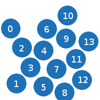
Now you can start busting. We check each particle with each other particle until the right border of the first particle is larger than the left border of the second particle.
Consider an example.
0 particle will check collision with 1 and 2:

1 with 2 and 3.
2 only with 3.
3 will check collision with 4, 5 and 6:
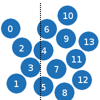
I think that the essence is clear.
My implementation of this algorithm is:
It should be noted that this algorithm is most effective in cases where the movement of particles in each moment of time is small, because the sorting takes the main load, and it will be performed faster if the particles are already partially sorted.
This algorithm can also be applied to more complex objects; in this case, use their AABB (Axis-Aligned Bounding Box, the minimum bounding box).
Complexity: O (n ^ 2) - in the worst case, O (n * log (n)) - on average
Pros:
* Easy to implement
* Not sensitive to different particle sizes.
* Good performance
Minuses:
* It takes a little time to understand the algorithm
As you probably already guessed from the name, the essence of the algorithm is reduced to the fact that the whole space is divided into a uniform network of small squares, the size of which is equal to the particle diameter. Each such square (cell) of this network is an array.
It may look, for example, like this:
At each iteration of the main loop, this network is cleared and refilled. The filling algorithm is extremely simple: the particle cell index is calculated by dividing both coordinates by the particle diameter and discarding the fractional part. Example:
Thus, for each particle it is necessary to calculate the index and enter it into the cell with this index (add an element to the array).
Now it only remains to go through each cell and check all its particles with all the particles of the neighboring 8 cells surrounding it, while not forgetting to check with itself.

This can be done like this:
Difficulty: O (n)
Pros:
* Fastest of all
* Easy to implement
Minuses:
* Requires additional memory
* Sensitive to different particle sizes (modification required)
This algorithm can be slightly improved by making a choice on which axis to sort the particles. The optimal axis is the one along which the largest number of particles are located.
Optimization number 1:
We use a more efficient network view:
I think it’s not necessary to say that a one-dimensional array is faster than a two-dimensional array, and also that a static array of constant length is faster than a dynamic std :: vector, not to mention that we merged all this. Just had to start another array, which will talk about how many particles are in each of the cells.
And yes, we have imposed a limit on the number of particles in a cell, and this is not very good, because threatens that with a strong squeeze, a much larger number of particles will have to be written into the cell, since this is impossible, some collisions will not be handled. However, with a good resolution of the collisions of this problem can be avoided.
Optimization number 2
Instead of completely clearing the grid array at each iteration of the main loop, we will only make the changes that have occurred.
We run over all the particles of each cell of the network, calculate the new particle index, and if it is not equal to the current one, then we remove the particle from the current cell and add it to the free space in the new cell.
Removal occurs by writing in its place the last particle from the same cell.
Here is my code that implements it:
Optimization number 3
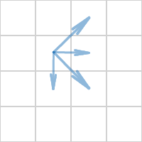
We use a check with the neighboring 8 cells. This is redundant, it is enough to check only 4 neighboring cells.
For example:
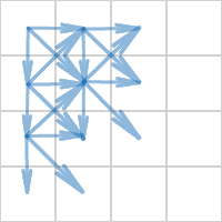
With the remaining cells, the test will pass either earlier or later:
Optimization number 4
You can speed up the algorithm a little by increasing the data locality in memory. This will allow more frequent reading of data from the processor cache, and less access to RAM. But do not do this at each iteration of the main loop, since this will kill all performance, however, you can perform this operation, for example, once a second, or once every few seconds if the scene changes slightly.
You can increase the locality by changing the order of the particles in the main array, in accordance with their location in the network.
Those. the first 4 particles will be from 0 cells, the next 4 from 1, and so on.
As can be seen from the table, the running time of the algorithms corresponds to their complexity, the regular network grows almost linearly :).
http://rghost.ru/35826275
The archive is a project written in CodeBlocks, as well as Linux binaries, but since I used the ClanLib library to create the window and display the graphics, then the project should compile without problems under Windows.
Program management:
number 1 - Bruteforce
figure 2 - Sweep & Prune
number 3 - Regulatory network
left mouse button - move "pushing".
This article provides a brief overview of the most common algorithms used to handle collisions. However, this does not limit the scope of these algorithms; nothing prevents them from being used for any other interaction. The main task that they take upon themselves is a more convenient presentation of data, in order to be able to quickly sift out pairs that are not interesting to us in advance.
For simplicity, we will consider the 2D case, the particles are round, the radius of the particles is the same for all.
Content
1. Overview of Algorithms
1.1. Brute force
1.2. Sweep & prune
1.3. Regular network
2. Some optimizations
2.1. Sweep & prune
2.2. Regular network
3. Comparison of execution speed
4. Application (program and source code)
5. Conclusion
')
1. Overview of Algorithms
1.1. Brute force
This is the easiest and at the same time the slowest of all possible ways. There is a check between all possible pairs of particles.
void Update() { for (int i = 0; i < NUM_P; ++i) { for (int j = i + 1; j < NUM_P; ++j) { Collision(&_particles[i], &_particles[j]); } } } Difficulty: O (n ^ 2)
Pros:
* Very easy to understand and implement.
* Not sensitive to different particle sizes.
Minuses:
* The slowest of all
1.2. Sweep & prune
The essence of this algorithm is that first we sort all the particles according to their left border along the OX axis, and then we check each particle only with those whose left border is less than the right edge of the current particle.
I will try to describe the operation of the algorithm in pictures.
Initial state:

As you can see, the particles are not ordered.
After sorting on the left border of the particle (position on X minus the radius of the particle), we get the following picture:

Now you can start busting. We check each particle with each other particle until the right border of the first particle is larger than the left border of the second particle.
Consider an example.
0 particle will check collision with 1 and 2:

1 with 2 and 3.
2 only with 3.
3 will check collision with 4, 5 and 6:

I think that the essence is clear.
My implementation of this algorithm is:
void Update() { qsort(_sap_particles, NUM_P, sizeof(Particle *), CompareParticles); for (int i = 0; i < NUM_P; ++i) { for (int j = i + 1; j < NUM_P && _sap_particles[i]->pos.x + RADIUS_P > _sap_particles[j]->pos.x - RADIUS_P; ++j) { Collision(_sap_particles[i], _sap_particles[j]); } } } It should be noted that this algorithm is most effective in cases where the movement of particles in each moment of time is small, because the sorting takes the main load, and it will be performed faster if the particles are already partially sorted.
This algorithm can also be applied to more complex objects; in this case, use their AABB (Axis-Aligned Bounding Box, the minimum bounding box).
Complexity: O (n ^ 2) - in the worst case, O (n * log (n)) - on average
Pros:
* Easy to implement
* Not sensitive to different particle sizes.
* Good performance
Minuses:
* It takes a little time to understand the algorithm
1.3. Regular network
As you probably already guessed from the name, the essence of the algorithm is reduced to the fact that the whole space is divided into a uniform network of small squares, the size of which is equal to the particle diameter. Each such square (cell) of this network is an array.
It may look, for example, like this:
const int _GRID_WIDTH = (int)(WIDTH / (RADIUS_P * 2.0f)); const int _GRID_HEIGHT = (int)(HEIGHT / (RADIUS_P * 2.0f)); std::vector<Particle *> _grid[_GRID_WIDTH][_GRID_HEIGHT]; At each iteration of the main loop, this network is cleared and refilled. The filling algorithm is extremely simple: the particle cell index is calculated by dividing both coordinates by the particle diameter and discarding the fractional part. Example:
int x = (int)(_particles[i].pos.x / (RADIUS_P * 2.0f)); int y = (int)(_particles[i].pos.y / (RADIUS_P * 2.0f)); Thus, for each particle it is necessary to calculate the index and enter it into the cell with this index (add an element to the array).
Now it only remains to go through each cell and check all its particles with all the particles of the neighboring 8 cells surrounding it, while not forgetting to check with itself.

This can be done like this:
void Update() { for (int i = 0; i < _GRID_WIDTH; ++i) { for (int j = 0; j < _GRID_HEIGHT; ++j) { _grid[i][j].clear(); } } for (int i = 0; i < MAX_P; ++i) { int x = (int)(_particles[i].pos.x / (RADIUS_P * 2.0f)); int y = (int)(_particles[i].pos.y / (RADIUS_P * 2.0f)); _grid[x][y].push_back(&_particles[i]); } // } Difficulty: O (n)
Pros:
* Fastest of all
* Easy to implement
Minuses:
* Requires additional memory
* Sensitive to different particle sizes (modification required)
2. Some optimizations
2.1. Sweep & prune
This algorithm can be slightly improved by making a choice on which axis to sort the particles. The optimal axis is the one along which the largest number of particles are located.
Optimum OY axis: | Optimum OX axis: |
2.2. Regular network
Optimization number 1:
We use a more efficient network view:
const int _MAX_CELL_SIZE = 4; const int _GRID_WIDTH = (int)(WIDTH / (RADIUS_P * 2.0f)); const int _GRID_HEIGHT = (int)(HEIGHT / (RADIUS_P * 2.0f)); int _cell_size[_GRID_WIDTH * _GRID_HEIGHT]; Particle *_grid[_GRID_WIDTH * _GRID_HEIGHT * _MAX_CELL_SIZE]; I think it’s not necessary to say that a one-dimensional array is faster than a two-dimensional array, and also that a static array of constant length is faster than a dynamic std :: vector, not to mention that we merged all this. Just had to start another array, which will talk about how many particles are in each of the cells.
And yes, we have imposed a limit on the number of particles in a cell, and this is not very good, because threatens that with a strong squeeze, a much larger number of particles will have to be written into the cell, since this is impossible, some collisions will not be handled. However, with a good resolution of the collisions of this problem can be avoided.
Optimization number 2
Instead of completely clearing the grid array at each iteration of the main loop, we will only make the changes that have occurred.
We run over all the particles of each cell of the network, calculate the new particle index, and if it is not equal to the current one, then we remove the particle from the current cell and add it to the free space in the new cell.
Removal occurs by writing in its place the last particle from the same cell.
Here is my code that implements it:
for (int i = 0; i < _GRID_WIDTH * _GRID_HEIGHT; ++i) { for (int j = 0; j < _cell_size[i]; ++j) { int x = (int)(_grid[i * _MAX_CELL_SIZE + j]->pos.x / (RADIUS_P * 2.0)); int y = (int)(_grid[i * _MAX_CELL_SIZE + j]->pos.y / (RADIUS_P * 2.0)); if (x < 0) { x = 0; } if (y < 0) { y = 0; } if (x >= _GRID_WIDTH) { x = _GRID_WIDTH - 1; } if (y >= _GRID_HEIGHT) { y = _GRID_HEIGHT - 1; } // if (x * _GRID_HEIGHT + y != i && _cell_size[x * _GRID_HEIGHT + y] < _MAX_CELL_SIZE) { _grid[(x * _GRID_HEIGHT + y) * _MAX_CELL_SIZE + _cell_size[x * _GRID_HEIGHT + y]++] = _grid[i * _MAX_CELL_SIZE + j]; // _grid[i * _MAX_CELL_SIZE + j] = _grid[i * _MAX_CELL_SIZE + --_cell_size[i]]; } } } Optimization number 3
We use a check with the neighboring 8 cells. This is redundant, it is enough to check only 4 neighboring cells.
For example:

With the remaining cells, the test will pass either earlier or later:

Optimization number 4
You can speed up the algorithm a little by increasing the data locality in memory. This will allow more frequent reading of data from the processor cache, and less access to RAM. But do not do this at each iteration of the main loop, since this will kill all performance, however, you can perform this operation, for example, once a second, or once every few seconds if the scene changes slightly.
You can increase the locality by changing the order of the particles in the main array, in accordance with their location in the network.
Those. the first 4 particles will be from 0 cells, the next 4 from 1, and so on.
3. Comparison of execution speed
| Number of particles | Bruteforce (ms) | Sweep & Prune (ms) | Regular network (ms) |
|---|---|---|---|
| 1000 | four | one | one |
| 2000 | 14 | one | one |
| 5000 | 89 | four | 2 |
| 10,000 | 355 | ten | four |
| 20,000 | 1438 | 28 | 7 |
| 30,000 | 3200 | 55 | eleven |
| 100,000 | 12737 | 140 | 23 |
As can be seen from the table, the running time of the algorithms corresponds to their complexity, the regular network grows almost linearly :).
4. Application (program and source code)
http://rghost.ru/35826275
The archive is a project written in CodeBlocks, as well as Linux binaries, but since I used the ClanLib library to create the window and display the graphics, then the project should compile without problems under Windows.
Program management:
number 1 - Bruteforce
figure 2 - Sweep & Prune
number 3 - Regulatory network
left mouse button - move "pushing".
5. Conclusion
This article provides a brief overview of the most common algorithms used to handle collisions. However, this does not limit the scope of these algorithms; nothing prevents them from being used for any other interaction. The main task that they take upon themselves is a more convenient presentation of data, in order to be able to quickly sift out pairs that are not interesting to us in advance.
Source: https://habr.com/ru/post/135948/
All Articles