Classical mechanics: about diffusions "on the fingers"
Recently looked at the Farseer Physics Engine . It became interesting how a dynamic object is implemented in this engine. As expected, I did not meet there the usual differential equations and their discrete realizations in the form of difference equations or discrete models of the state space. The main excuse is the declared reason for the abandonment of “fair” mechanics in many gaming physics engines - the excessive complexity of working with differential equations and too much computational load.
In this article, I continue the topic of digital signal processing. In it, I will try to speak in simple language about the concept of game mechanics (physics) using an approach based on differential equations. In the future, I am going to assess whether the implementation of such an approach will really lead to a sharp increase in the computational load. In the framework of this article will not work - too much. In this I am going to describe the purpose of the coefficients included in the mathematical model of a dynamic object, to describe their physical meaning, i.e. their influence on the behavior of a dynamic object.
Perhaps we will start ...
In my article about the Kalman Filter, I described what the “input-output” equations are, the transfer function, and the operator form for writing differential equations (see the section “Basic concepts” in [2]). The following equation can serve as an example of a part of a mathematical model of a dynamic object in the operator record form:
(one)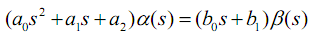
This is a common simplified model of dynamic systems. Ahead of it, I will write that the body model in the Farseer engine uses a stripped-down analog of the model presented above (second-order dynamic link). Below is a description of the notation adopted in it.
The presented equation describes a dynamic system of the type “single input - single output” (SISO). It can be used to describe the dynamics of an object according to one of its degrees of freedom. As you may know, a free body has six degrees of freedom - three translational (linear motion along the three axes of the coordinate system (SC)) and three rotational (turns around the axes of the SC). Thus, the complete model of the physical body will be described by six such equations (or four for the 2D case). You can immediately say that this already indicates that the approach is too complex. But in fact, in Farseer, for example, the body class (Body) contains both the linear coordinates of the body (essentially, it is the α (s) pair for OX and OY), and the linear velocities (the s * α (s) pair for OX and OY) ) and orientation parameters and angular velocity. These parameters are calculated separately for each of the axes, i.e. the number of equations is the same - two equations along the axis OX (linear and angular motion) and two for the axis OY. The only difference is in the form of equations.
The algorithm in the Farseer engine is approximate and simplified, but it allows you to work with varying time slices. The function of calculation of motion parameters ( Island.Solve (ref TimeStep step, ref Vector2 gravity) ) transmits the time elapsed after the last calculation of parameters. This allows, with insufficient computer performance, to keep the flow rate of game time approximately constant to the detriment of the smoothness and realism of the movement of game objects.
When constructing a discrete model based on differential equations, we clearly tie in to a fixed time quantum. The equations are integrated for the initially specified discretization rate, and if since the last calculation, for some reason, more time has passed than the specified quantum (in the English literature it is called “time sample”), then we must either calculate several times, or we will get a slowdown the movement of the object. Last I just watched in the game " Command Cortex " on a weak machine. The movements of the actors were smooth but slow (the actors controlled by man gain an advantage). Thus, one cannot speak of the exceptional advantage of one of these approaches.
Now, about what the coefficients of the above equation are responsible for. This equation describes the movement of the physical body relative to its equilibrium position with α (s) = 0. This is another reason for the seeming inconvenience of using such a model in game mechanics. In the absence of applied external forces, this model will sooner or later return (if the model is stable) the body to an equilibrium position. Imagine a game world filled with balls that all the time tend to the origin (for example, to the upper left corner of the screen). The presence of a stiffness coefficient leads to this behavior (see a2 above). Imagine that the body is connected to the origin of the spring. While forces act on the body, the spring is stretched, but it is necessary to remove the external effect and the body will rush to zero. The bodies in the Farseer engine do not have this behavior. If we set the coefficient a2 to zero, then in this case the bodies will not tend to the origin of coordinates (see above, I wrote that the models in Farseer are in fact trimmed versions of this model). Well, why is this coefficient then needed, you ask. If you open the brackets on the left side of equation (1) and instead of the addend
a2 * α (s)
write
a2 * (α (s) - α0)
then through α0 we will be able to set the position to which the game object will strive. The magnitude of the coefficient a2 is responsible for how quickly the body moves to a given equilibrium position (the higher the value, the higher the spring stiffness). How this is implemented in Farseer, I have not yet figured out, but I think I will have to create an additional source of impact.
Now the coefficient a1. This is the damping coefficient. The greater the value of this coefficient, the faster the speed is quenched (linear or angular). Life analogy - viscous liquids such as oil, honey, epoxy resin. These fluids are very viscous (the damping coefficient is very important). The higher the speed of movement of the body in them, the higher the resistance to this movement. If you slowly move a spoon in them, for example, you will not be able to overcome the resistance of big work, but if you strike with a swing, then the blow will be tough.
The value of the coefficient a0 characterizes the inertia of the object. In describing linear motion, mass is used as the coefficient a0. The higher its value, the slower the body picks up speed when external forces are applied to it.
Now about the coefficients on the right side of equation (1). It should be noted here that this model is extended to the case when the input action is determined not only by the value of the external force itself, but also by its change. To describe the dynamics of game objects, this may be superfluous. However, in industrial systems management there are also such models. What is their physical meaning? The coefficient b1 is essentially the coefficient of transfer of external force into the object. It is usually equal to one unit, i.e. power is transmitted as is.
The coefficient b0 is interesting. It plays the role of a forcing factor. Imagine a very inertial object to which a force is applied that gradually increases with time. If the rate of increase and the final magnitude of the force will be small, then the object is very slowly gaining speed. But if a force is made large, then after an external force reaches a given value, the object will not stop in some position, but will oscillate under the action of inertia. Forcing is an impact proportional to the rate of increase of external force. If we choose a large one, then even at a low rate of increase in external force, our object will pick up speed fairly quickly, and when the external force reaches the specified value, the boost will turn off. Here is such a cunning this "b0".
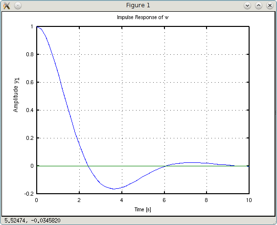
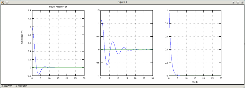
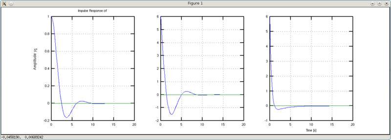
To clearly show the effect of diff factors. equations for the behavior of a dynamic object decided to construct graphs of the transition process with step response and impulse response input effects. A total of 6 groups of graphs are presented (one group for each coefficient). The graphs are built in the Octave package (v. 3.4) with the “Signal Processing” package installed.
So, let's take the model of the form as the initial one:
=========================================
>>> w = tf ([1 1], [1 1 1])
')
Transfer function "w" from input "u1" to output ...
y1: (s + 1) / (s ^ 2 + s + 1)
Continuous-time model.
=========================================

The code "w = tf ([1 1], [1 1 1])" in symbolic form is:
>>> w = tf ([b0 b1], [a0 a1 a2])
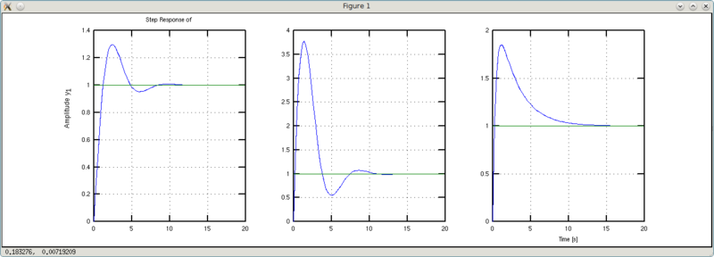
In the screenshots at the bottom right, the approximate stabilization time (the stability corridor is ± 5% of the specified value).
Let's try to play with the stiffness coefficient a2.
>>> w1 = 0.1 * tf ([1 1], [1 1 0.1])
y1: (s + 1) / (s ^ 2 + s + 0.1)
>>> w2 = 10 * tf ([1 1], [1 1 10])
y1: (s + 1) / (s ^ 2 + s + 10)
Note: it was necessary to podshamanit with gain factors so that the resulting gain factor was equal to one.
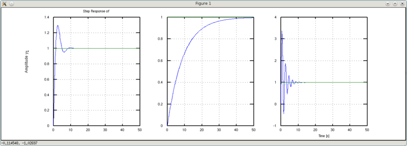

What can be seen on the charts? From left to right are graphs for w, w1 and w2, respectively. The w1 plots are smoother and more slowly reach steady-state values. The w2 plots are more oscillatory in nature, but reach a steady-state value more quickly. Conclusion: stiffer spring - more oscillations, but a shorter transition process.
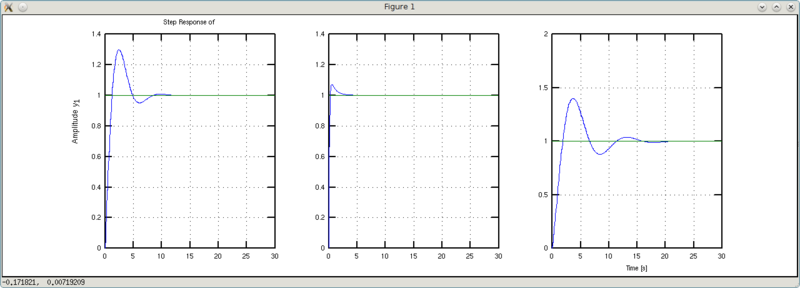
Let's try to play with damping (a1).
>>> w1 = tf ([1 1], [1 0.25 1])
y1: (s + 1) / (s ^ 2 + 0.25s + 1)
>>> w2 = tf ([1 1], [1 2 1])
y1: (s + 1) / (s ^ 2 + 2s + 1)
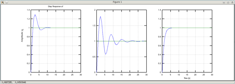
Immediately conclusion: more viscosity - oscillations damp out faster.
Let's try to play with inertia (a0).
>>> w1 = tf ([1 1], [0.1 1 1])
y1: (s + 1) / (0.1s ^ 2 + s + 1)
>>> w2 = tf ([1 1], [2 1 1])
y1: (s + 1) / (2s ^ 2 + s + 1)
Conclusion: the weight of the cast iron is less - less turbulence and a shorter transition process.
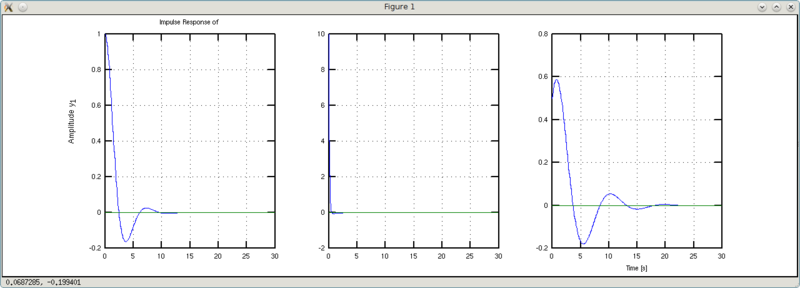
We turn to the right side and play with b1.
>>> w1 = 10 * tf ([1 0.1], [1 1 1])
y1: (10 s + 1) / (s ^ 2 + s + 1)
>>> w2 = 0.25 * tf ([1 4], [1 1 1])
y1: (0.25 s + 1) / (s ^ 2 + s + 1)

It seems that the difference is barely noticeable when you look at the Step Response graphics. But on the Impulse Response graphs, the effect of this coefficient is clearly visible. If it is equal to one, then the pulse transition process starts from one (in fact, it goes out of zero, but it doesn’t matter - the second value in the unit graph). The graph w1 “starts” from the value 10 (the reciprocal of 0.1), and the graph w2 starts from the value 0.25 (inverse to 4). Thus, the coefficient b1 can be “denounced” by the coefficient of management efficiency (input action).
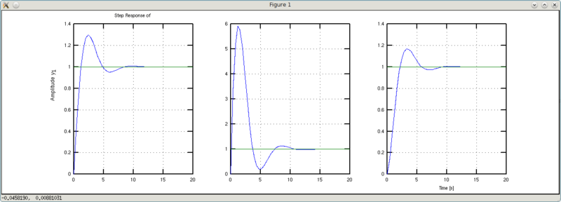
And finally, delicious - games with coefficient b0. This is a tricky ratio, because the comparison will not be as it was above. To show its effect will have to vary several factors.
>>> w1 = tf ([6 1], [1 1 1])
y1: (6 s + 1) / (s ^ 2 + s + 1)
>>> w2 = tf ([6 1], [1 3 1])
y1: (6 s + 1) / (s ^ 2 + 3 s + 1)
What is the difference between w1 and w2? W2 has three times the damping coefficient. As a result, we get interesting conclusions. Graphs w1 and w2 cross the steady-state level earlier than the default graph. However, the w1 graph retains the default form with its oscillation, while the w2 graph retains a more smoothed due to the increased damping. Thus, playing with forcing and damping, we can make even a cast iron iron flit around the ring like a butterfly without hesitation to and fro.
In this article I considered only positive values of the coefficients. Their positivity is a necessary condition for the stability of the mat. models. However, you can try to play with negative values. An unstable system can also be controlled. Think of the fifth generation aircraft (for example, our Golden Eagle). The reverse sweep of the wing is an unstable glider, but on the other hand, it has high maneuverability. Automation is able to correct this instability and at the same time, when necessary, lay steep turns.
If it works out, I'll concoct a toy with which you can visually see all these effects.
Introduction
In this article, I continue the topic of digital signal processing. In it, I will try to speak in simple language about the concept of game mechanics (physics) using an approach based on differential equations. In the future, I am going to assess whether the implementation of such an approach will really lead to a sharp increase in the computational load. In the framework of this article will not work - too much. In this I am going to describe the purpose of the coefficients included in the mathematical model of a dynamic object, to describe their physical meaning, i.e. their influence on the behavior of a dynamic object.
Perhaps we will start ...
Physical sense
In my article about the Kalman Filter, I described what the “input-output” equations are, the transfer function, and the operator form for writing differential equations (see the section “Basic concepts” in [2]). The following equation can serve as an example of a part of a mathematical model of a dynamic object in the operator record form:
(one)
This is a common simplified model of dynamic systems. Ahead of it, I will write that the body model in the Farseer engine uses a stripped-down analog of the model presented above (second-order dynamic link). Below is a description of the notation adopted in it.
- a0, a1, a2 are the coefficients of inertia, damping and stiffness, respectively.
- b0, b1 - input factors.
- s is the Laplass operator (d / dt).
- α (s), β (s) are the output and input variables, as functions of the Laplass operator.
The presented equation describes a dynamic system of the type “single input - single output” (SISO). It can be used to describe the dynamics of an object according to one of its degrees of freedom. As you may know, a free body has six degrees of freedom - three translational (linear motion along the three axes of the coordinate system (SC)) and three rotational (turns around the axes of the SC). Thus, the complete model of the physical body will be described by six such equations (or four for the 2D case). You can immediately say that this already indicates that the approach is too complex. But in fact, in Farseer, for example, the body class (Body) contains both the linear coordinates of the body (essentially, it is the α (s) pair for OX and OY), and the linear velocities (the s * α (s) pair for OX and OY) ) and orientation parameters and angular velocity. These parameters are calculated separately for each of the axes, i.e. the number of equations is the same - two equations along the axis OX (linear and angular motion) and two for the axis OY. The only difference is in the form of equations.
The algorithm in the Farseer engine is approximate and simplified, but it allows you to work with varying time slices. The function of calculation of motion parameters ( Island.Solve (ref TimeStep step, ref Vector2 gravity) ) transmits the time elapsed after the last calculation of parameters. This allows, with insufficient computer performance, to keep the flow rate of game time approximately constant to the detriment of the smoothness and realism of the movement of game objects.
When constructing a discrete model based on differential equations, we clearly tie in to a fixed time quantum. The equations are integrated for the initially specified discretization rate, and if since the last calculation, for some reason, more time has passed than the specified quantum (in the English literature it is called “time sample”), then we must either calculate several times, or we will get a slowdown the movement of the object. Last I just watched in the game " Command Cortex " on a weak machine. The movements of the actors were smooth but slow (the actors controlled by man gain an advantage). Thus, one cannot speak of the exceptional advantage of one of these approaches.
Now, about what the coefficients of the above equation are responsible for. This equation describes the movement of the physical body relative to its equilibrium position with α (s) = 0. This is another reason for the seeming inconvenience of using such a model in game mechanics. In the absence of applied external forces, this model will sooner or later return (if the model is stable) the body to an equilibrium position. Imagine a game world filled with balls that all the time tend to the origin (for example, to the upper left corner of the screen). The presence of a stiffness coefficient leads to this behavior (see a2 above). Imagine that the body is connected to the origin of the spring. While forces act on the body, the spring is stretched, but it is necessary to remove the external effect and the body will rush to zero. The bodies in the Farseer engine do not have this behavior. If we set the coefficient a2 to zero, then in this case the bodies will not tend to the origin of coordinates (see above, I wrote that the models in Farseer are in fact trimmed versions of this model). Well, why is this coefficient then needed, you ask. If you open the brackets on the left side of equation (1) and instead of the addend
a2 * α (s)
write
a2 * (α (s) - α0)
then through α0 we will be able to set the position to which the game object will strive. The magnitude of the coefficient a2 is responsible for how quickly the body moves to a given equilibrium position (the higher the value, the higher the spring stiffness). How this is implemented in Farseer, I have not yet figured out, but I think I will have to create an additional source of impact.
Now the coefficient a1. This is the damping coefficient. The greater the value of this coefficient, the faster the speed is quenched (linear or angular). Life analogy - viscous liquids such as oil, honey, epoxy resin. These fluids are very viscous (the damping coefficient is very important). The higher the speed of movement of the body in them, the higher the resistance to this movement. If you slowly move a spoon in them, for example, you will not be able to overcome the resistance of big work, but if you strike with a swing, then the blow will be tough.
The value of the coefficient a0 characterizes the inertia of the object. In describing linear motion, mass is used as the coefficient a0. The higher its value, the slower the body picks up speed when external forces are applied to it.
Now about the coefficients on the right side of equation (1). It should be noted here that this model is extended to the case when the input action is determined not only by the value of the external force itself, but also by its change. To describe the dynamics of game objects, this may be superfluous. However, in industrial systems management there are also such models. What is their physical meaning? The coefficient b1 is essentially the coefficient of transfer of external force into the object. It is usually equal to one unit, i.e. power is transmitted as is.
The coefficient b0 is interesting. It plays the role of a forcing factor. Imagine a very inertial object to which a force is applied that gradually increases with time. If the rate of increase and the final magnitude of the force will be small, then the object is very slowly gaining speed. But if a force is made large, then after an external force reaches a given value, the object will not stop in some position, but will oscillate under the action of inertia. Forcing is an impact proportional to the rate of increase of external force. If we choose a large one, then even at a low rate of increase in external force, our object will pick up speed fairly quickly, and when the external force reaches the specified value, the boost will turn off. Here is such a cunning this "b0".
Dynamics in pictures
To clearly show the effect of diff factors. equations for the behavior of a dynamic object decided to construct graphs of the transition process with step response and impulse response input effects. A total of 6 groups of graphs are presented (one group for each coefficient). The graphs are built in the Octave package (v. 3.4) with the “Signal Processing” package installed.
So, let's take the model of the form as the initial one:
=========================================
>>> w = tf ([1 1], [1 1 1])
')
Transfer function "w" from input "u1" to output ...
y1: (s + 1) / (s ^ 2 + s + 1)
Continuous-time model.
=========================================
The code "w = tf ([1 1], [1 1 1])" in symbolic form is:
>>> w = tf ([b0 b1], [a0 a1 a2])
In the screenshots at the bottom right, the approximate stabilization time (the stability corridor is ± 5% of the specified value).
Let's try to play with the stiffness coefficient a2.
>>> w1 = 0.1 * tf ([1 1], [1 1 0.1])
y1: (s + 1) / (s ^ 2 + s + 0.1)
>>> w2 = 10 * tf ([1 1], [1 1 10])
y1: (s + 1) / (s ^ 2 + s + 10)
Note: it was necessary to podshamanit with gain factors so that the resulting gain factor was equal to one.
What can be seen on the charts? From left to right are graphs for w, w1 and w2, respectively. The w1 plots are smoother and more slowly reach steady-state values. The w2 plots are more oscillatory in nature, but reach a steady-state value more quickly. Conclusion: stiffer spring - more oscillations, but a shorter transition process.
Let's try to play with damping (a1).
>>> w1 = tf ([1 1], [1 0.25 1])
y1: (s + 1) / (s ^ 2 + 0.25s + 1)
>>> w2 = tf ([1 1], [1 2 1])
y1: (s + 1) / (s ^ 2 + 2s + 1)
Immediately conclusion: more viscosity - oscillations damp out faster.
Let's try to play with inertia (a0).
>>> w1 = tf ([1 1], [0.1 1 1])
y1: (s + 1) / (0.1s ^ 2 + s + 1)
>>> w2 = tf ([1 1], [2 1 1])
y1: (s + 1) / (2s ^ 2 + s + 1)
Conclusion: the weight of the cast iron is less - less turbulence and a shorter transition process.
We turn to the right side and play with b1.
>>> w1 = 10 * tf ([1 0.1], [1 1 1])
y1: (10 s + 1) / (s ^ 2 + s + 1)
>>> w2 = 0.25 * tf ([1 4], [1 1 1])
y1: (0.25 s + 1) / (s ^ 2 + s + 1)
It seems that the difference is barely noticeable when you look at the Step Response graphics. But on the Impulse Response graphs, the effect of this coefficient is clearly visible. If it is equal to one, then the pulse transition process starts from one (in fact, it goes out of zero, but it doesn’t matter - the second value in the unit graph). The graph w1 “starts” from the value 10 (the reciprocal of 0.1), and the graph w2 starts from the value 0.25 (inverse to 4). Thus, the coefficient b1 can be “denounced” by the coefficient of management efficiency (input action).
And finally, delicious - games with coefficient b0. This is a tricky ratio, because the comparison will not be as it was above. To show its effect will have to vary several factors.
>>> w1 = tf ([6 1], [1 1 1])
y1: (6 s + 1) / (s ^ 2 + s + 1)
>>> w2 = tf ([6 1], [1 3 1])
y1: (6 s + 1) / (s ^ 2 + 3 s + 1)
What is the difference between w1 and w2? W2 has three times the damping coefficient. As a result, we get interesting conclusions. Graphs w1 and w2 cross the steady-state level earlier than the default graph. However, the w1 graph retains the default form with its oscillation, while the w2 graph retains a more smoothed due to the increased damping. Thus, playing with forcing and damping, we can make even a cast iron iron flit around the ring like a butterfly without hesitation to and fro.
As PS
In this article I considered only positive values of the coefficients. Their positivity is a necessary condition for the stability of the mat. models. However, you can try to play with negative values. An unstable system can also be controlled. Think of the fifth generation aircraft (for example, our Golden Eagle). The reverse sweep of the wing is an unstable glider, but on the other hand, it has high maneuverability. Automation is able to correct this instability and at the same time, when necessary, lay steep turns.
If it works out, I'll concoct a toy with which you can visually see all these effects.
Sources
- Game physics engine " Farseer "
- Kalman filter - is it difficult?
Source: https://habr.com/ru/post/135794/
All Articles