Draw pictures using the Hilbert curve
On Saturday last week, “it was evening, there was nothing to do,” and the sourcerer habloiser and I did not understand what it was talking about. And for some reason, we are talking about a problem inverse to the task of constructing a graph of a function by its expression. That is, for example, we have the expression y ( x ) = (cos 0.5 x ⋅ cos 200 x + | x | 0.5 - 0.7) (4 - x 2 ) 0.01 . The graph of such a function is somewhat reminiscent of a heart . 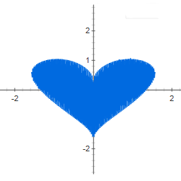 But we were interested in the reverse question, how, having, for example, an image of a heart, get an expression for a function whose graph would be this very heart.
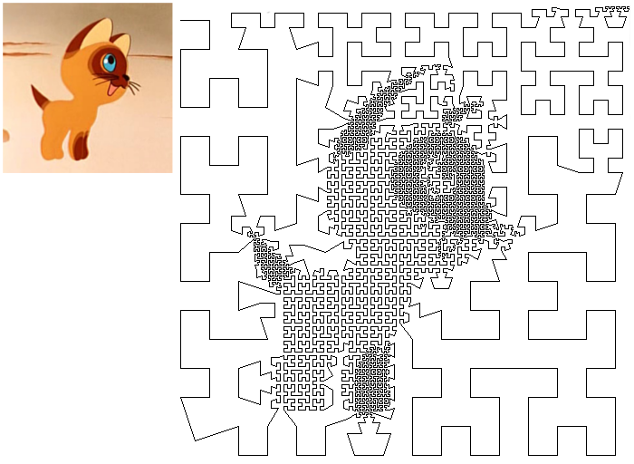
I didn’t want to remember any rows of Fourier, but I wanted something simple and beautiful. We began to recall known results related to this issue. The result was a program that generates a broken line in the image that is somewhat similar to the original image. Using the example of a kitten named Gav, it looks like this (look better from afar):
')
If you are interested in how to do this, as well as learn about the formula of hemp, a formula whose schedule is the same formula, then welcome to Habrakat. (There will be a lot of pictures.)
So, let's recall some results.
Formula hemp . Around 2005, the hemp formula was actively developed and discussed . Simple formulas in polar coordinates of the form
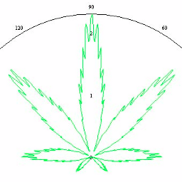
What did Anton Sukhinov do? In 2005, at the watermelon forum, he suggested the following intricate formula (if I was not mistaken when typing anywhere):
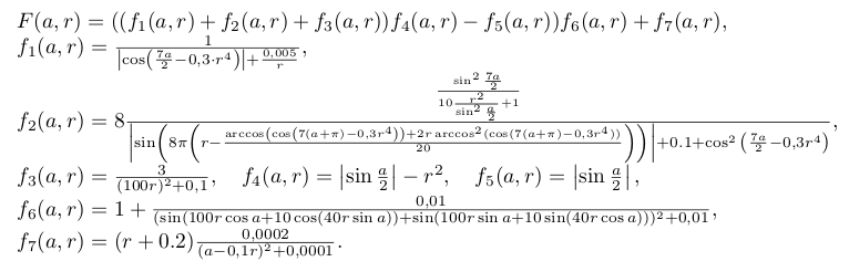
Then, drawing only those points for which F ( a , r )> 0 and choosing the color depending on the value of the function, we get the following image:

Jump off the mind, is not it?
Tupper Formula . Consider the inequality
 and let the number k be
48584506361897134235820959624942020445814005879832445494830930850619347
04708809928450644769865524364849997247024915119110411605739177407856919
75432657185544205721044573588368182982375413963433822519945219165128434
83329051311931999535024137587652392648746133949068701305622958132194811
13685339535565290850023875092856892694555974281546386510730049106723058
93358605254409666435126534936364395712556569593681518433485760526694016
12512669514215505395545191537854575257565907405401579290017659679654800
64427829131488548259914721248506352686630476300.
It turns out that the set of points ( x , y - k ) satisfying this inequality and such that 0 ≤ x ≤ 106 and k ≤ y ≤ k + 17, looks like this:

And this is inequality itself again. It is clear, of course, that the image is simply encrypted in the number k , but nevertheless the result is very beautiful and it is not clear how such a thing could have been thought up.
More details can be found in Wikipedia: Tupper's self-referential formula , and we will move from private results to mass methods.
Systems of iterated functions. Probably everyone who has come across fractals at least a little bit knows what a system of iterative functions is. CIF allows using a pair of tens of numbers to get pictures very similar to real leaves, trees, branches:
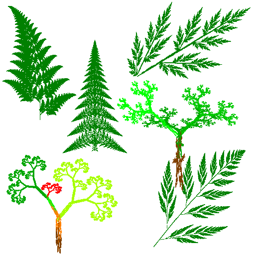
The idea that you can try to solve the inverse problem - for a given image to get a set of numbers describing the CIF, allowed Michael Barnsley to come up with fractal compression . Some attempt to talk about fractal compression has already been made in Habré: Fundamentals of fractal image compression . But for those who want to understand in detail, I will recommend the first half of the book Fractals and Wavelets for Compressing Images in Action by S. Welstead.
Fractal lines . In fact, the fractal compression algorithm uses not systems of iterative functions, but so-called systems of partial iterative functions. Nevertheless, there is a class of images for which it is easy to come up with exactly CIF, of which they are attractors. Such images are fractal lines. A fractal line is a word, each letter of which consists of reduced copies of a given word and so on. On the example of the word "HABR" it looks something like this:
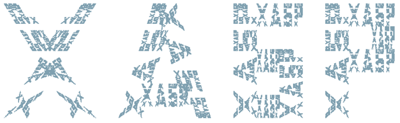
It is easy to understand how to do this for an arbitrary word, just spend a little time to represent each word as a set of parallelograms. At least five years ago it was done. A detailed description and code can be found in the article Fractal lines .
Portrait of V.-J. Möller. Leafing through the book Fractals, Chaos, Power Laws. Miniatures from the infinite paradise "M. Schroeder, you can stumble upon the following illustration:
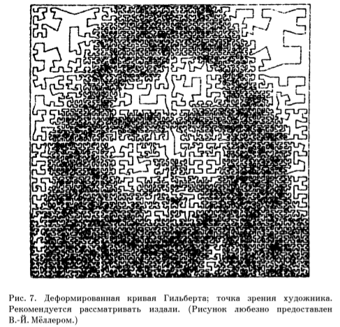
It looks very nice, and it is clear that this can be done with an arbitrary image. About how it was drawn, the book is not told, but not difficult to guess for yourself.
First you need to take the algorithm for constructing the Hilbert curve. But not with the help of any L-systems, but an honest recursive algorithm. And then we modify it as follows. If the brightness of a square is greater than a predetermined threshold, and in its four sub-squares there is no need to draw a curve, then we consider that there is no need to draw a curve in the box itself. Although it's probably easier to understand from the code below.
Before the image was fed to the program, it was translated into shades of gray and empirically adjusted the brightness and contrast. For example, this is what happened when the program was set on Tux:

The source code of the program.
If someone knows any other beautiful results from the discussed area, then write about it, please, in the comments.
But we were interested in the reverse question, how, having, for example, an image of a heart, get an expression for a function whose graph would be this very heart.I didn’t want to remember any rows of Fourier, but I wanted something simple and beautiful. We began to recall known results related to this issue. The result was a program that generates a broken line in the image that is somewhat similar to the original image. Using the example of a kitten named Gav, it looks like this (look better from afar):
')
If you are interested in how to do this, as well as learn about the formula of hemp, a formula whose schedule is the same formula, then welcome to Habrakat. (There will be a lot of pictures.)
So, let's recall some results.
Formula hemp . Around 2005, the hemp formula was actively developed and discussed . Simple formulas in polar coordinates of the form
- R ( t ) = (1 + sin t ) (1 + 0.9 ⋅ cos 8 t ) (1 + 0.1 ⋅ cos 24 t ),
- R ( t ) = (1 + sin t ) (1 - 0.9 ⋅ | sin 4t |) ⋅ (0.9 + 0.05 ⋅ cos 200 t ),
- R ( t ) = (1 + sin t ) (1 + 0.9 ⋅ cos 8 t ) (1 + 0.1 ⋅ cos 24 t ) (0.5 + 0.05 ⋅ cos 140 t )
What did Anton Sukhinov do? In 2005, at the watermelon forum, he suggested the following intricate formula (if I was not mistaken when typing anywhere):
Then, drawing only those points for which F ( a , r )> 0 and choosing the color depending on the value of the function, we get the following image:
Jump off the mind, is not it?
Tupper Formula . Consider the inequality
and let the number k be48584506361897134235820959624942020445814005879832445494830930850619347
04708809928450644769865524364849997247024915119110411605739177407856919
75432657185544205721044573588368182982375413963433822519945219165128434
83329051311931999535024137587652392648746133949068701305622958132194811
13685339535565290850023875092856892694555974281546386510730049106723058
93358605254409666435126534936364395712556569593681518433485760526694016
12512669514215505395545191537854575257565907405401579290017659679654800
64427829131488548259914721248506352686630476300.
It turns out that the set of points ( x , y - k ) satisfying this inequality and such that 0 ≤ x ≤ 106 and k ≤ y ≤ k + 17, looks like this:
And this is inequality itself again. It is clear, of course, that the image is simply encrypted in the number k , but nevertheless the result is very beautiful and it is not clear how such a thing could have been thought up.
More details can be found in Wikipedia: Tupper's self-referential formula , and we will move from private results to mass methods.
Systems of iterated functions. Probably everyone who has come across fractals at least a little bit knows what a system of iterative functions is. CIF allows using a pair of tens of numbers to get pictures very similar to real leaves, trees, branches:
The idea that you can try to solve the inverse problem - for a given image to get a set of numbers describing the CIF, allowed Michael Barnsley to come up with fractal compression . Some attempt to talk about fractal compression has already been made in Habré: Fundamentals of fractal image compression . But for those who want to understand in detail, I will recommend the first half of the book Fractals and Wavelets for Compressing Images in Action by S. Welstead.
Fractal lines . In fact, the fractal compression algorithm uses not systems of iterative functions, but so-called systems of partial iterative functions. Nevertheless, there is a class of images for which it is easy to come up with exactly CIF, of which they are attractors. Such images are fractal lines. A fractal line is a word, each letter of which consists of reduced copies of a given word and so on. On the example of the word "HABR" it looks something like this:
It is easy to understand how to do this for an arbitrary word, just spend a little time to represent each word as a set of parallelograms. At least five years ago it was done. A detailed description and code can be found in the article Fractal lines .
Portrait of V.-J. Möller. Leafing through the book Fractals, Chaos, Power Laws. Miniatures from the infinite paradise "M. Schroeder, you can stumble upon the following illustration:
It looks very nice, and it is clear that this can be done with an arbitrary image. About how it was drawn, the book is not told, but not difficult to guess for yourself.
First you need to take the algorithm for constructing the Hilbert curve. But not with the help of any L-systems, but an honest recursive algorithm. And then we modify it as follows. If the brightness of a square is greater than a predetermined threshold, and in its four sub-squares there is no need to draw a curve, then we consider that there is no need to draw a curve in the box itself. Although it's probably easier to understand from the code below.
Point2D[] drawHilbertCurve(Point2D p, double size, int d) { Point2D q = new Point2D.Double( p.getX() + size * sqrt(2) * cos(PI * (d + 0.5) / 2), p.getY() + size * sqrt(2) * sin(PI * (d + 0.5) / 2)); if (size <= 2) { if (blockIsWhite(p, q)) { return null; } else { Point2D cc = new Point2D.Double( p.getX() + size * sqrt(2) * cos(PI * (d + 0.5) / 2) / 2, p.getY() + size * sqrt(2) * sin(PI * (d + 0.5) / 2) / 2); return new Point2D[]{cc, cc}; } } else { Point2D cl = new Point2D.Double( p.getX() + size * cos(PI * (d + 1) / 2) / 2, p.getY() + size * sin(PI * (d + 1) / 2) / 2); Point2D cc = new Point2D.Double( p.getX() + size * sqrt(2) * cos(PI * (d + 0.5) / 2) / 2, p.getY() + size * sqrt(2) * sin(PI * (d + 0.5) / 2) / 2); Point2D br = new Point2D.Double( p.getX() + size * cos(PI * d / 2), p.getY() + size * sin(PI * d / 2)); Point2D[] p1 = drawHilbertCurve(cl, size / 2, d - 1); Point2D[] p2 = drawHilbertCurve(cl, size / 2, d); Point2D[] p3 = drawHilbertCurve(cc, size / 2, d); Point2D[] p4 = drawHilbertCurve(br, size / 2, d + 1); if (p1 == null && p2 == null && p3 == null && p4 == null && blockIsWhite(p, q)) { return null; } else { if (p1 == null) { p1 = new Point2D[2]; p1[0] = p1[1] = new Point2D.Double( cl.getX() + size * sqrt(2) * cos(PI * (d - 0.5) / 2) / 4, cl.getY() + size * sqrt(2) * sin(PI * (d - 0.5) / 2) / 4); } if (p2 == null) { p2 = new Point2D[2]; p2[0] = p2[1] = new Point2D.Double( cl.getX() + size * sqrt(2) * cos(PI * (d + 0.5) / 2) / 4, cl.getY() + size * sqrt(2) * sin(PI * (d + 0.5) / 2) / 4); } if (p3 == null) { p3 = new Point2D[2]; p3[0] = p3[1] = new Point2D.Double( cc.getX() + size * sqrt(2) * cos(PI * (d + 0.5) / 2) / 4, cc.getY() + size * sqrt(2) * sin(PI * (d + 0.5) / 2) / 4); } if (p4 == null) { p4 = new Point2D[2]; p4[0] = p4[1] = new Point2D.Double( br.getX() + size * sqrt(2) * cos(PI * (d + 1.5) / 2) / 4, br.getY() + size * sqrt(2) * sin(PI * (d + 1.5) / 2) / 4); } drawLine(p1[0], p2[0]); drawLine(p2[1], p3[0]); drawLine(p3[1], p4[1]); } return new Point2D[]{p1[1], p4[0]}; } } boolean blockIsWhite(Point2D p, Point2D q) { int l = (int) min(p.getX(), q.getX()); int r = (int) max(p.getX(), q.getX()); int t = (int) min(p.getY(), q.getY()); int b = (int) max(p.getY(), q.getY()); double c = 0; for (int i = l; i < r; ++i) { for (int j = t; j < b; ++j) { c += (srcImage.getRGB(i, j) & 0x0000FF) / 255.0; } } return c / ((b - t) * (r - l)) > threshold * (1 - log(2) / log(b - t)); } Before the image was fed to the program, it was translated into shades of gray and empirically adjusted the brightness and contrast. For example, this is what happened when the program was set on Tux:
The source code of the program.
If someone knows any other beautiful results from the discussed area, then write about it, please, in the comments.
Source: https://habr.com/ru/post/135344/
All Articles