What is a hidden Markov model
In recognition, signals are often thought of as multiplication products that act statistically. Thus, the purpose of analyzing such signals is to model the static properties of signal sources as accurately as possible. The basis of this model is a simple study of the data and the possible degree of restriction of the deviations that occur. However, the model to be determined should not only repeat the generation of certain data as precisely as possible, but also deliver useful information about some significant units for the segmentation of signals.
Hidden Markov models are able to handle both of the above aspects of the simulation. In a two-stage stochastic process, information for segmentation can be obtained from the internal states of the model, while the data signal itself is generated in the second stage.
This modeling technology gained great popularity as a result of successful application and further development in the field of automatic speech recognition. Research on hidden Markov models has surpassed all competing approaches, and are the dominant processing paradigm. Their ability to describe processes or signals has been successfully studied for a long time. The reason for this, in particular, is the fact that the technology for constructing artificial neural networks is rarely used for speech recognition and similar segmentation problems. Nevertheless, there are a number of hybrid systems consisting of a combination of hidden Markov models and artificial neural networks in which they take advantage of both modeling methods (see section 5.8.2).
')
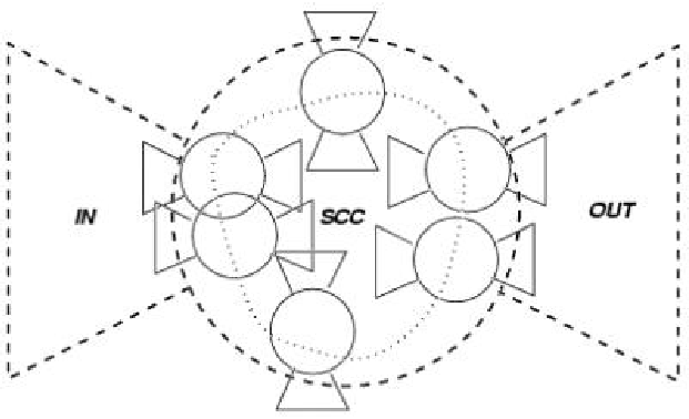
Hidden Markov models (SMM) describe a two-stage stochastic process. The first stage consists of a discrete stochastic process that is static, causative and simple. The state space is considered as final. Thus, the process probabilistically describes the state of transition to discreteness, the finite state space. This can be visualized as a finite automaton with differences between any pairs of states that are labeled with a transition probability. The behavior of the process at a given time t depends only on the immediate state of the preceding element and can be characterized as follows:
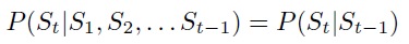
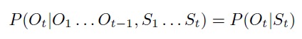
At the second stage, for each time point t, additionally, by output or output data, Ot is generated. The propagation of associative probability depends only on the current state of St, and not on any previous states or output data.
This sequence of output data is the only thing that can be observed in the behavior of the model. On the other hand, the sequence state received during data generation cannot be examined. This is the so-called “stealth”, from which the definition of hidden Markov models is derived. If you look at the model externally - that is, to observe its behavior - quite often there are references to a sequence of output states Oi, O2 ... OT, as the reason for observing the sequence. Further, the individual elements of this sequence will be called the result of observation.
In the literature, patterns of recognition of the behavior of the SMM are always considered at a certain time interval T. To initialize the model at the beginning of this period, additional probabilities are used to describe the probability distribution of states at time t = 1. The equivalent criterion for the final state is usually absent. Thus, the actions of the model come to an end state as soon as an arbitrary state is reached at the time point T. Neither static nor declarative criteria are used to more accurately mark the end of states.
However, the hidden Markov models of the first order, which are usually designated as A, are fully described:
• establishment of a finite set of states {s | 1 <s <N}, in the literature, as a rule, only their indices are called,
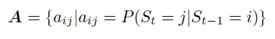
• state of transition probabilities, matrix A
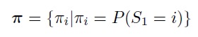
• vector of the beginning of states π
• state of a specific probability distribution
 f for model output
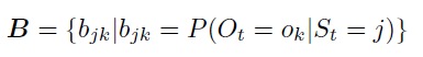
However, the distribution of the output must be distinguished depending on the type of output during generation. In the simplest case, the output data is generated from discrete probability distributions {O1, O2 ... OM}, and therefore, they are of character type. The parameter bj (ok) represents the discrete distribution probability, which can be grouped into an output probability matrix:
With this choice of simulation output, the so-called discrete HMM is obtained.
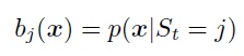
If, when there is a vector of sequence values xe IRn, and not the output of the distribution data described on the basis of the continuous probability distribution function:
The current use of the SMM for signal analysis tasks is used exclusively by the so-called continuous SMM, although the need to simulate continuous distribution greatly increases the complexity of the analysis.
Translation of Chapter 5 (1 paragraph)
Gernot A. Fink "Markov Models for Pattern Recognition From Theory to Applications"
Hidden Markov models are able to handle both of the above aspects of the simulation. In a two-stage stochastic process, information for segmentation can be obtained from the internal states of the model, while the data signal itself is generated in the second stage.
This modeling technology gained great popularity as a result of successful application and further development in the field of automatic speech recognition. Research on hidden Markov models has surpassed all competing approaches, and are the dominant processing paradigm. Their ability to describe processes or signals has been successfully studied for a long time. The reason for this, in particular, is the fact that the technology for constructing artificial neural networks is rarely used for speech recognition and similar segmentation problems. Nevertheless, there are a number of hybrid systems consisting of a combination of hidden Markov models and artificial neural networks in which they take advantage of both modeling methods (see section 5.8.2).
Definition
')
Hidden Markov models (SMM) describe a two-stage stochastic process. The first stage consists of a discrete stochastic process that is static, causative and simple. The state space is considered as final. Thus, the process probabilistically describes the state of transition to discreteness, the finite state space. This can be visualized as a finite automaton with differences between any pairs of states that are labeled with a transition probability. The behavior of the process at a given time t depends only on the immediate state of the preceding element and can be characterized as follows:
At the second stage, for each time point t, additionally, by output or output data, Ot is generated. The propagation of associative probability depends only on the current state of St, and not on any previous states or output data.
This sequence of output data is the only thing that can be observed in the behavior of the model. On the other hand, the sequence state received during data generation cannot be examined. This is the so-called “stealth”, from which the definition of hidden Markov models is derived. If you look at the model externally - that is, to observe its behavior - quite often there are references to a sequence of output states Oi, O2 ... OT, as the reason for observing the sequence. Further, the individual elements of this sequence will be called the result of observation.
In the literature, patterns of recognition of the behavior of the SMM are always considered at a certain time interval T. To initialize the model at the beginning of this period, additional probabilities are used to describe the probability distribution of states at time t = 1. The equivalent criterion for the final state is usually absent. Thus, the actions of the model come to an end state as soon as an arbitrary state is reached at the time point T. Neither static nor declarative criteria are used to more accurately mark the end of states.
However, the hidden Markov models of the first order, which are usually designated as A, are fully described:
• establishment of a finite set of states {s | 1 <s <N}, in the literature, as a rule, only their indices are called,
• state of transition probabilities, matrix A
• vector of the beginning of states π
• state of a specific probability distribution
f for model outputHowever, the distribution of the output must be distinguished depending on the type of output during generation. In the simplest case, the output data is generated from discrete probability distributions {O1, O2 ... OM}, and therefore, they are of character type. The parameter bj (ok) represents the discrete distribution probability, which can be grouped into an output probability matrix:
With this choice of simulation output, the so-called discrete HMM is obtained.
If, when there is a vector of sequence values xe IRn, and not the output of the distribution data described on the basis of the continuous probability distribution function:
The current use of the SMM for signal analysis tasks is used exclusively by the so-called continuous SMM, although the need to simulate continuous distribution greatly increases the complexity of the analysis.
Translation of Chapter 5 (1 paragraph)
Gernot A. Fink "Markov Models for Pattern Recognition From Theory to Applications"
Source: https://habr.com/ru/post/135281/
All Articles