Dynamic programming in speech recognition algorithms
In speech recognition systems that contain words, recognition requires a comparison between the input word and the various words in the dictionary. The effective solution of the problem lies in the dynamic comparison algorithms, the purpose of which is to introduce the time scales of two words into optimal correspondence. Algorithms of this type are dynamic timeline transformation algorithms. This article presents two variants of the implementation of the algorithm designed to recognize individual words.
Studies in the field of speech recognition, as well as in other areas, follow two directions: fundamental research, the purpose of which is to develop and test new methods, algorithms and concepts on a non-commercial basis; and applied research, which aims to improve existing methods by following certain criteria. This article discusses the recognition of individual words in the trend of applied research.
')
Basic research is aimed at obtaining a medium or long-term benefit, while applied research is aimed at rapidly improving existing methods or expanding their use in areas where such methods are practically not used.
Improving the speed of speech recognition can be given the following criteria:
Today, sound recognition systems are built on the basis of the recognition principles of recognition forms. The methods and algorithms that have been used so far can be divided into four large classes:
Discriminative analysis methods based on Bayesian discrimination;
Hidden Markov models;
Dynamic programming - temporary dynamic algorithms (DTW);
Neural networks;
This article provides an example and alternative to the DTW dynamic programming algorithm that implements speech recognition.
Dynamic Time Transformation Algorithm (DTW)
The dynamic time transformation (DTW) algorithm calculates the optimal sequence of time transformation (deformation) between two time series. The algorithm calculates both strain values between two rows and the distance between them.
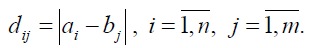
Suppose we have two numerical sequences (a1, a2, ..., an) and (b1, b2, ..., bm). As you can see, the length of the two sequences may be different. The algorithm begins with calculating local deviations between elements of two sequences that use different types of deviations. The most common method for calculating deviations is the method that calculates the absolute deviation between the values of two elements (Euclidean distance). As a result, we obtain a deviation matrix with n rows and m columns of common members:
The minimum distance in the matrix between the sequences is determined using a dynamic programming algorithm and the following optimization criterion:
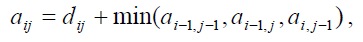
where: aij is the minimum distance between the sequences (a1, a2, ..., an) and (b1, b2, ..., bm). The deformation path is the minimum distance in the matrix between the elements a11 and anm, consisting of those aij elements that express the distance to anm.
Global deformations consist of two sequences and are determined by the following formula:

where: wi - elements that belong to the strain path; p is their number. The calculations were made for two short sequences and are shown in the table in which the strain sequence is highlighted.

There are three conditions imposed on the DTW algorithm to ensure fast convergence:
1. Monotonicity - the path never returns, that is: both indices, i and j, which are used in a sequence, never decrease.
2. Continuity - the sequence advances gradually: in one step, the indices, i and j, increase by no more than 1.
3. Limit - the sequence begins in the lower left corner and ends in the upper right.
An example of sequence deformation using the Java programming language is shown below:
Since to determine the basis of a sequence in dynamic programming, it is optimal to use the inverse programming method, it is necessary to use a certain dynamic type of structure called a “stack”. Like any dynamic programming algorithm, DWT has a polynomial complexity. When we deal with large sequences, there are two disadvantages:
- Memorization of large numeric matrices;
- Perform a large number of calculations of deviations.
There is an improved version of the algorithm, FastDWT, which solves the above two problems. The solution is to split the state matrix into 2, 4, 8, 16, etc. smaller matrices by repeating the process of splitting the input sequence into two parts. Thus, deviations are calculated only on these small matrices, and the deformation paths calculated for small matrices. From the algorithmic point of view, the proposed solution is based on the “Divide et Impera” method (approx. Trans. From the Latin. “Divide and dominate”).
The sound passes through the medium, as a longitudinal wave with a velocity depending on the density of the medium. The easiest way to present sounds is a sine graph. Graphic representation of the air vibrations under pressure for some time.
The shape of the sound wave depends on three factors: aplitude, frequency, and phase.
Amplitude is the movement of sinusoidal graphs above and below the time axis (y = 0), which corresponds to the energy of the loaded sound wave. Amplitude measurements can be made in pressure units (DB decibels), which measure the amplitude of normal sound using logarithmic functions. Measuring amplitude using decibels is very important in practice, as it is a direct idea of how the sound volume is perceived by people. Frequency - the number of sinusoid cycles per second. The cycle of oscillations begins with the middle line, then reaches a maximum and a minimum, and then returns to the middle line. The cycle frequency is measured in one second or in hertz (Hz). The inverse of the frequency is called the period - the time required for the sound wave to complete the cycle.
The last factor is the phase. It measures the position relative to the start of the sine curve. A phase cannot be heard by a person, but it can be defined relative to the position between two signals. However, the hearing aid perceives the position of the sound on different phases.
In order to parse the sound waves on a sinusoidal curve, we use the Fourier theorem. It states that any complex periodic wave can be disassembled using a sinusoidal curve with different frequencies, amplitudes and phases. This process is called Fourier analysis, and its result is a set of amplitudes, phases and frequencies for each sinusoidal wave component. Putting these sinusoidal curves together, we get the original sound wave. The point of frequency or phase taken together with amplitude is called a spectrum. Any periodic signal indicates a recursive model of time, which corresponds to the first frequency of the signal and is called the fundamental frequency. It can be measured from a speech signal by checking the period of oscillation around the 0 axis. The spectrum shows the frequency of a short sequence of sounds, and if we want to analyze its development over time, you need to find a way to demonstrate this. This can be shown on the spectrogram. A spectrogram is a diagram in two dimensions: frequency and time, in which the color of a point (dark - strong, bright - weak) determines the amplitude of the intensity. The method plays an important role in speech recognition, and a professional can reveal many details by looking only at the sound spectrogram.
Modern detection methods can accurately determine the starting and ending point of the spoken word in the audio stream, based on signal processing that changes over time. These methods estimate the energy and the average value in a short period of time, and also calculate the average level of zero crossing.
Creating a start and end point is a simple task if the audio recording is done under ideal conditions. In this case, the signal-to-noise ratio is great, since it is not difficult to determine the actual signal in the stream by analyzing the images. In reality, everything is not so simple: the background noise is of tremendous intensity and can disrupt the process of separating words in a stream of speech.
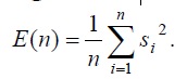
The best word separation algorithm is the Rabinel-Lamel algorithm. If we consider Stob pulses {s1, s2, ..., sn}, where n is the number of strobe pulse images, and si, i = 1, n is the numerical expression of the samples, the total strobe pulse energy is calculated:
Middle level zero crossing:
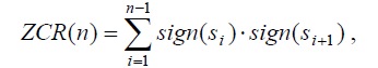
Where:
The method uses three numeric levels: two for energy (upper, lower) and one for the average zero crossing. The point from which energy overlaps the upper level and the level of positive and negative values does not cancel the set level, which is considered the starting point of the voice sound (not silence). The search for the first such point is made by crossing the pulses from the beginning to the end, and this will determine the first area with speech. The reverse transition, from end to beginning, allows you to determine the end point of the last area with the speech. The definition within the region can be made by crossing the pulses between these two points. The onset of the deaf region begins at the point at which the energy becomes less than the value of the lower level. Pay attention to the figure below, in which before and after the removal of the blind area:
beep the words "nouă"
Definition of words using the DWT algorithm
The definition of a word can be done by comparing numerical waveforms or by comparing the spectrogram of signals. The comparison process in both cases should compensate for the different sequence lengths and the non-linear nature of the sound. The DWT algorithm manages to sort out these problems by finding the deformation corresponding to the optimal distance between two rows of different lengths.
There are 2 features of the algorithm:
1. Direct comparison of numerical waveforms. In this case, for each numerical sequence, a new sequence is created, the dimensions of which are much smaller. The algorithm deals with these sequences. A numeric sequence can have several thousand numeric values, while a subsequence can have several hundred values. Reducing the number of numerical values can be accomplished by removing them between the corner points. This process of reducing the length of a numerical sequence should not change its presentation. Undoubtedly, the process leads to a decrease in recognition accuracy. However, taking into account the increase in speed, accuracy, in fact, is increased by increasing the words in the dictionary.
2. Representation of spectrogram signals and application of the DTW algorithm for comparing two spectrograms. The method consists in dividing a digital signal into a number of intervals that will overlap. For each pulse, the intervals of real numbers (sound frequencies) will calculate the Fast Fourier Transform, and will be stored in the matrix of the sound spectrogram. The parameters will be the same for all computational operations: pulse lengths, Fourier transform lengths, overlap lengths for two consecutive pulses. The Fourier transform is symmetrically related to the center, and the complex number is on the one hand related to the numbers on the other. In this regard, only the values from the first part of the symmetry can be saved, so the spectrogram will represent the matrix of complex numbers, the number of lines in such a matrix is equal to half the length of the Fourier transform, and the number of columns will be determined depending on the length of the sound. DTW will be applied on the matrix of real numbers as a result of conjugation of the spectrogram of values, such a matrix is called the energy matrix.
DTW algorithms are very useful for recognizing individual words in a limited vocabulary. For recognition of fluent speech, hidden Markov models are used. The use of dynamic programming provides the polymineral complexity of the algorithm: O (n2v), where n is the length of the sequence, and v is the number of words in the dictionary.
DWT have several weaknesses. First, O (n2v) complexity does not satisfy large dictionaries, which increase the success of the recognition process. Secondly, it is difficult to calculate two elements in two different sequences, if we take into account that there are many channels with different characteristics. However, DTW remains simple to implement, open to improvements and suitable for applications that require simple word recognition: telephones, car computers, security systems, etc.
[1] Benoit Legrand, CS Chang, SH Ong, Soek-Ying Neo, Nallasivam Palanisamy, Chromosome classification using dynamic time warping, ScienceDirect Pattern Recognition Letters 29 (2008) 215–222
[2] Cory Myers, Lawyers R. Rabiner, Aaron E. Rosenberg, Word Logging Recognition, Ieee Transactions On Acoustics, Speech, And Signal Processing, Vol. Assp-28, No. 6, December 1980
[3] F. Jelinek. “Continuous Speech Recognition by Statisical Methods.” IEEE Proceedings 64: 4 (1976): 532-556
[4] Rabiner, LR, A Tutorial on Hidden Markov Models and Selected Applications in Speech Recognition, Proc. of IEEE, Feb. 1989
[5] Rabiner, LR, Schafer, RW, Digital Processing of Speech Signals, Prentice Hall, 1978.
[6] Stan Salvador, Chan, FastDTW: Toward Accurate Dynamic Time Warping in Linear Time
and Space, IEEE Transactions on Biomedical. Engineering, vol. 43, no. four
[7] Young, S., A Review of Large-Vocabulary Continuous Speech Recognition, IEEE Signal
Processing Magazine, pp. 45-57, Sep. 1996
[8] Sakoe, H. & S. Chiba. (1978) Dynamic programming optimization for spoken word recognition. IEEE Trans. Acoustics, Speech, and Signal Proc., Vol. ASSP-26.
[9] Furtună, F., Dârdală, M., Using Discriminant of the Fourth National Conference Humman Computer Interaction 2007, Universitatea Ovidius ConstanRa, 2007, MatrixRom, Bucharest, 2007
[10] * * *, Speech Separation by Humans, Kluwer Academic Publishers, 2005
article translation: Dynamic Programming Algorithms in Speech Recognition by Titus Felix FURTUNĂ
Introduction
Studies in the field of speech recognition, as well as in other areas, follow two directions: fundamental research, the purpose of which is to develop and test new methods, algorithms and concepts on a non-commercial basis; and applied research, which aims to improve existing methods by following certain criteria. This article discusses the recognition of individual words in the trend of applied research.
')
Basic research is aimed at obtaining a medium or long-term benefit, while applied research is aimed at rapidly improving existing methods or expanding their use in areas where such methods are practically not used.
Improving the speed of speech recognition can be given the following criteria:
- The size of recognizable vocabulary;
- The degree of spontaneity of speech that must be recognized;
- Addiction / independence from announcer;
- The time required to set the system in motion;
- System adjustment time for new users;
- Time selection and recognition;
- The degree of recognition (expressed by word or sentence).
Today, sound recognition systems are built on the basis of the recognition principles of recognition forms. The methods and algorithms that have been used so far can be divided into four large classes:
Discriminative analysis methods based on Bayesian discrimination;
Hidden Markov models;
Dynamic programming - temporary dynamic algorithms (DTW);
Neural networks;
This article provides an example and alternative to the DTW dynamic programming algorithm that implements speech recognition.
Dynamic Time Transformation Algorithm (DTW)
The dynamic time transformation (DTW) algorithm calculates the optimal sequence of time transformation (deformation) between two time series. The algorithm calculates both strain values between two rows and the distance between them.
Suppose we have two numerical sequences (a1, a2, ..., an) and (b1, b2, ..., bm). As you can see, the length of the two sequences may be different. The algorithm begins with calculating local deviations between elements of two sequences that use different types of deviations. The most common method for calculating deviations is the method that calculates the absolute deviation between the values of two elements (Euclidean distance). As a result, we obtain a deviation matrix with n rows and m columns of common members:
The minimum distance in the matrix between the sequences is determined using a dynamic programming algorithm and the following optimization criterion:
where: aij is the minimum distance between the sequences (a1, a2, ..., an) and (b1, b2, ..., bm). The deformation path is the minimum distance in the matrix between the elements a11 and anm, consisting of those aij elements that express the distance to anm.
Global deformations consist of two sequences and are determined by the following formula:
where: wi - elements that belong to the strain path; p is their number. The calculations were made for two short sequences and are shown in the table in which the strain sequence is highlighted.
There are three conditions imposed on the DTW algorithm to ensure fast convergence:
1. Monotonicity - the path never returns, that is: both indices, i and j, which are used in a sequence, never decrease.
2. Continuity - the sequence advances gradually: in one step, the indices, i and j, increase by no more than 1.
3. Limit - the sequence begins in the lower left corner and ends in the upper right.
An example of sequence deformation using the Java programming language is shown below:
public static void dtw(double a[],double b[],double dw[][], Stack<Double> w){ // a,b - the sequences, dw - the minimal distances matrix // w - the warping path int n=a.length,m=b.length; double d[][]=new double[n][m]; // the euclidian distances matrix for(int i=0;i<n;i++) for(int j=0;j<m;j++)d[i][j]=Math.abs(a[i]-b[j]); // determinate of minimal distance dw[0][0]=d[0][0]; for(int i=1;i<n;i++)dw[i][0]=d[i][0]+dw[i-1][0]; for(int j=1;j<m;j++)dw[0][j]=d[0][j]+dw[0][j-1]; for(int i=1;i<n;i++) for(int j=1;j<m;j++) if(dw[i-1][j-1]<=dw[i-1][j]) if(dw[i-1][j-1]<=dw[i][j-1])dw[i][j]=d[i][j]+dw[i-1][j-1]; else dw[i][j]=d[i][j]+dw[i][j-1]; else if(dw[i-1][j]<=dw[i][j-1])dw[i][j]=d[i][j]+dw[i-1][j]; else dw[i][j]=d[i][j]+dw[i][j-1]; int i=n-1,j=m-1; double element=dw[i][j]; // determinate of warping path w.push(new Double(dw[i][j])); do{ if(i>0&&j>0) if(dw[i-1][j-1]<=dw[i-1][j]) if(dw[i-1][j-1]<=dw[i][j-1]){i--;j--;} else j--; else if(dw[i-1][j]<=dw[i][j-1])i--; else j--; else if(i==0)j--; else i--; w.push(new Double(dw[i][j])); } while(i!=0||j!=0); }Since to determine the basis of a sequence in dynamic programming, it is optimal to use the inverse programming method, it is necessary to use a certain dynamic type of structure called a “stack”. Like any dynamic programming algorithm, DWT has a polynomial complexity. When we deal with large sequences, there are two disadvantages:
- Memorization of large numeric matrices;
- Perform a large number of calculations of deviations.
There is an improved version of the algorithm, FastDWT, which solves the above two problems. The solution is to split the state matrix into 2, 4, 8, 16, etc. smaller matrices by repeating the process of splitting the input sequence into two parts. Thus, deviations are calculated only on these small matrices, and the deformation paths calculated for small matrices. From the algorithmic point of view, the proposed solution is based on the “Divide et Impera” method (approx. Trans. From the Latin. “Divide and dominate”).
Using DWT Algorithm in Speech Recognition
Voice Signal Analysis
The sound passes through the medium, as a longitudinal wave with a velocity depending on the density of the medium. The easiest way to present sounds is a sine graph. Graphic representation of the air vibrations under pressure for some time.
The shape of the sound wave depends on three factors: aplitude, frequency, and phase.
Amplitude is the movement of sinusoidal graphs above and below the time axis (y = 0), which corresponds to the energy of the loaded sound wave. Amplitude measurements can be made in pressure units (DB decibels), which measure the amplitude of normal sound using logarithmic functions. Measuring amplitude using decibels is very important in practice, as it is a direct idea of how the sound volume is perceived by people. Frequency - the number of sinusoid cycles per second. The cycle of oscillations begins with the middle line, then reaches a maximum and a minimum, and then returns to the middle line. The cycle frequency is measured in one second or in hertz (Hz). The inverse of the frequency is called the period - the time required for the sound wave to complete the cycle.
The last factor is the phase. It measures the position relative to the start of the sine curve. A phase cannot be heard by a person, but it can be defined relative to the position between two signals. However, the hearing aid perceives the position of the sound on different phases.
In order to parse the sound waves on a sinusoidal curve, we use the Fourier theorem. It states that any complex periodic wave can be disassembled using a sinusoidal curve with different frequencies, amplitudes and phases. This process is called Fourier analysis, and its result is a set of amplitudes, phases and frequencies for each sinusoidal wave component. Putting these sinusoidal curves together, we get the original sound wave. The point of frequency or phase taken together with amplitude is called a spectrum. Any periodic signal indicates a recursive model of time, which corresponds to the first frequency of the signal and is called the fundamental frequency. It can be measured from a speech signal by checking the period of oscillation around the 0 axis. The spectrum shows the frequency of a short sequence of sounds, and if we want to analyze its development over time, you need to find a way to demonstrate this. This can be shown on the spectrogram. A spectrogram is a diagram in two dimensions: frequency and time, in which the color of a point (dark - strong, bright - weak) determines the amplitude of the intensity. The method plays an important role in speech recognition, and a professional can reveal many details by looking only at the sound spectrogram.
Identify words
Modern detection methods can accurately determine the starting and ending point of the spoken word in the audio stream, based on signal processing that changes over time. These methods estimate the energy and the average value in a short period of time, and also calculate the average level of zero crossing.
Creating a start and end point is a simple task if the audio recording is done under ideal conditions. In this case, the signal-to-noise ratio is great, since it is not difficult to determine the actual signal in the stream by analyzing the images. In reality, everything is not so simple: the background noise is of tremendous intensity and can disrupt the process of separating words in a stream of speech.
The best word separation algorithm is the Rabinel-Lamel algorithm. If we consider Stob pulses {s1, s2, ..., sn}, where n is the number of strobe pulse images, and si, i = 1, n is the numerical expression of the samples, the total strobe pulse energy is calculated:
Middle level zero crossing:
Where:
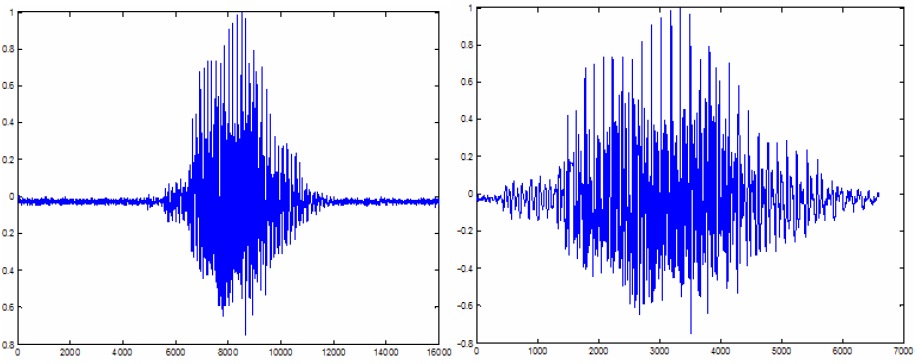
The method uses three numeric levels: two for energy (upper, lower) and one for the average zero crossing. The point from which energy overlaps the upper level and the level of positive and negative values does not cancel the set level, which is considered the starting point of the voice sound (not silence). The search for the first such point is made by crossing the pulses from the beginning to the end, and this will determine the first area with speech. The reverse transition, from end to beginning, allows you to determine the end point of the last area with the speech. The definition within the region can be made by crossing the pulses between these two points. The onset of the deaf region begins at the point at which the energy becomes less than the value of the lower level. Pay attention to the figure below, in which before and after the removal of the blind area:
beep the words "nouă"
Definition of words using the DWT algorithm
The definition of a word can be done by comparing numerical waveforms or by comparing the spectrogram of signals. The comparison process in both cases should compensate for the different sequence lengths and the non-linear nature of the sound. The DWT algorithm manages to sort out these problems by finding the deformation corresponding to the optimal distance between two rows of different lengths.
There are 2 features of the algorithm:
1. Direct comparison of numerical waveforms. In this case, for each numerical sequence, a new sequence is created, the dimensions of which are much smaller. The algorithm deals with these sequences. A numeric sequence can have several thousand numeric values, while a subsequence can have several hundred values. Reducing the number of numerical values can be accomplished by removing them between the corner points. This process of reducing the length of a numerical sequence should not change its presentation. Undoubtedly, the process leads to a decrease in recognition accuracy. However, taking into account the increase in speed, accuracy, in fact, is increased by increasing the words in the dictionary.
2. Representation of spectrogram signals and application of the DTW algorithm for comparing two spectrograms. The method consists in dividing a digital signal into a number of intervals that will overlap. For each pulse, the intervals of real numbers (sound frequencies) will calculate the Fast Fourier Transform, and will be stored in the matrix of the sound spectrogram. The parameters will be the same for all computational operations: pulse lengths, Fourier transform lengths, overlap lengths for two consecutive pulses. The Fourier transform is symmetrically related to the center, and the complex number is on the one hand related to the numbers on the other. In this regard, only the values from the first part of the symmetry can be saved, so the spectrogram will represent the matrix of complex numbers, the number of lines in such a matrix is equal to half the length of the Fourier transform, and the number of columns will be determined depending on the length of the sound. DTW will be applied on the matrix of real numbers as a result of conjugation of the spectrogram of values, such a matrix is called the energy matrix.
Conclusion
DTW algorithms are very useful for recognizing individual words in a limited vocabulary. For recognition of fluent speech, hidden Markov models are used. The use of dynamic programming provides the polymineral complexity of the algorithm: O (n2v), where n is the length of the sequence, and v is the number of words in the dictionary.
DWT have several weaknesses. First, O (n2v) complexity does not satisfy large dictionaries, which increase the success of the recognition process. Secondly, it is difficult to calculate two elements in two different sequences, if we take into account that there are many channels with different characteristics. However, DTW remains simple to implement, open to improvements and suitable for applications that require simple word recognition: telephones, car computers, security systems, etc.
Literature
[1] Benoit Legrand, CS Chang, SH Ong, Soek-Ying Neo, Nallasivam Palanisamy, Chromosome classification using dynamic time warping, ScienceDirect Pattern Recognition Letters 29 (2008) 215–222
[2] Cory Myers, Lawyers R. Rabiner, Aaron E. Rosenberg, Word Logging Recognition, Ieee Transactions On Acoustics, Speech, And Signal Processing, Vol. Assp-28, No. 6, December 1980
[3] F. Jelinek. “Continuous Speech Recognition by Statisical Methods.” IEEE Proceedings 64: 4 (1976): 532-556
[4] Rabiner, LR, A Tutorial on Hidden Markov Models and Selected Applications in Speech Recognition, Proc. of IEEE, Feb. 1989
[5] Rabiner, LR, Schafer, RW, Digital Processing of Speech Signals, Prentice Hall, 1978.
[6] Stan Salvador, Chan, FastDTW: Toward Accurate Dynamic Time Warping in Linear Time
and Space, IEEE Transactions on Biomedical. Engineering, vol. 43, no. four
[7] Young, S., A Review of Large-Vocabulary Continuous Speech Recognition, IEEE Signal
Processing Magazine, pp. 45-57, Sep. 1996
[8] Sakoe, H. & S. Chiba. (1978) Dynamic programming optimization for spoken word recognition. IEEE Trans. Acoustics, Speech, and Signal Proc., Vol. ASSP-26.
[9] Furtună, F., Dârdală, M., Using Discriminant of the Fourth National Conference Humman Computer Interaction 2007, Universitatea Ovidius ConstanRa, 2007, MatrixRom, Bucharest, 2007
[10] * * *, Speech Separation by Humans, Kluwer Academic Publishers, 2005
article translation: Dynamic Programming Algorithms in Speech Recognition by Titus Felix FURTUNĂ
Source: https://habr.com/ru/post/135087/
All Articles