What is artificial neural networks?
Artificial neural networks are used in various fields of science: from speech recognition systems to recognition of the secondary structure of a protein, the classification of various types of cancer and genetic engineering. However, how do they work and how are they good?
When it comes to tasks other than processing large amounts of information, the human brain has a great advantage over the computer. A person can recognize faces, even if there are many extraneous objects and poor lighting in the room. We easily understand strangers even when we are in a noisy room. But, despite years of research, computers are still far from performing similar tasks at a high level.
The human brain is surprisingly reliable: compared to a computer, it will not stop working just because a few cells will die, while the computer usually does not sustain any breakdowns in the CPU. But the most amazing feature of the human brain is that it can learn. No software and no updates are needed if we want to learn to ride a bike.
')
Brain calculations are made using closely interconnected neural networks that transmit information by sending electrical impulses through neural wiring consisting of axons, synapses, and dendrites. In 1943, McCulloch and Pitts modeled an artificial neuron, like a switch that receives information from other neurons and, depending on the total weighted input, is either activated or remains inactive. In the ANN node, the incoming signals are multiplied by the corresponding synapse weights and summed. These factors can be both positive (exciting) and negative (inhibiting). In the 1960s, it was proved that such neural models have properties similar to the brain: they can perform complex pattern recognition operations, and they can function even if some connections between neurons are broken. The demonstration of the percepton Rosenblatt showed that simple networks of such neurons can be trained on examples known in certain areas. Later, Minsky and Papert proved that simple prepeptons can solve only a very narrow class of linearly separable problems (see below), after which the activity of studying the ANN decreased. Nevertheless, the method of back propagation of a learning error, which can facilitate the task of learning complex neural networks with examples, has shown that these problems may not be separable.
The NETtalk program used artificial neural networks for machine-readable text and was the first widely known application. In biology, exactly the same type of network was used to predict the secondary structure of a protein; in fact, some of the best researchers still use the same method. From this another wave began, which aroused interest in the research of the INS and raised the hype around the magical training of thinking machines. Some of the most important early discoveries are from source 5.
ANNs can be created by simulating a model of neuron networks on a computer. Using algorithms that mimic the processes of real neurons, we can make the network "learn", which helps to solve many different problems. The neuron model is represented as a threshold value (it is illustrated in Figure 1a). The model receives data from a number of other external sources, determines the value of each input and adds these values. If the total input is above the threshold value, then the output of the block is equal to one, otherwise - zero. Thus, the output changes from 0 to 1 when the total “weighted” sum of the inputs is equal to the threshold value. Points in the original space that satisfy this condition determine the so-called hyperplanes. In two dimensions, the hyperplane is a line, while in three dimensions, the hyperplane is a normal (perpendicular) plane. The points on one side of the hyperplane are classified as 0, and the points on the other side are 1. This means that the classification problem can be solved using a threshold value if the two classes are separated by a hyperplane. These problems are called linearly separable and are depicted in Figure 1b.
picture 1
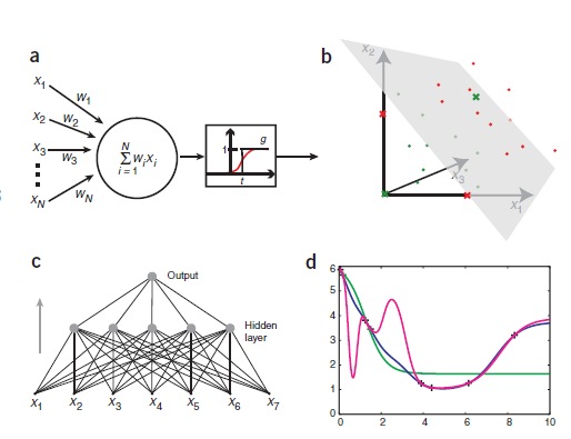
Artificial neural networks. (a) A graphical representation of the neural network model and the McCulloch and Pitts threshold element. The threshold block receives input from N other blocks or external sources, numbered from 1 to N. The input i is called xi and is associated with the weight wi. The total input to the device to measure the sum of weights over all inputs, wixi = w1x1 + w2x2 +.. + WNxΣi = 1 N N. be expressed as wixi Σi = 1 - tg (N), where g is a step function, which is 0 if the argument is negative, and 1 if the argument is positive (the actual value in nele does not matter, here, we chose 1). The so-called transfer function, g, can also be uninterrupted and “sigmoidal,” as indicated by the red line. (b) Linear separability (separability). In three dimensions, the threshold value can classify moments that can be separated by a plane. Each point represents the input value x1, x2, x3 at the threshold of the block. The green dots correspond to the data points of class 0, and the red dots represent 1. The green and red crosses illustrate the logical function of the exclusive or. It is impossible to find planes that separate green and red points (or lines in x1, x2, planes). (C) Unidirectional ANN. The shown network occupies seven entrances, has five units in a hidden layer and one exit. This is a two-layer network, because the input layer does not make any changes and is not taken into account. (d) retraining. Eight points are shown as pluses on a parabola (with the exception of “experimental” noise). They are used to train three different ANNs. Networks perceive x values as input (one input) and learn with y value as the desired result. As expected, the network with one hidden unit (green) does not cope with high-level work. The network with 10 hidden elements (blue) brings the basic functions surprisingly well. The last network with 20 hidden elements (purple) processes information well, the network is well trained, but for some intermediate areas it is overly creative.
If the classification problem is separable, then we still need to find a way to establish the weight and the threshold value so that the threshold device solves the classification problem correctly. This can be achieved by constantly adding examples from a previously known classification. This process is called learning or training, as it resembles the process of learning something by man. Simulation of computer-assisted learning implies a constant change in weights and thresholds in such a way that the classification gets a higher level after each step. The training can be implemented by various algorithms, we will talk about one of these algorithms later.
During training, the hyperplane moves in one direction, then in another, until it finds the correct position in space, after which it will not change significantly. Such a process is well demonstrated by the Neural Java program ( http://lcn.epfl.ch/tutorial/english/index.html ); Follow the link “Adline, Percepton and Backpropagation” (the red and blue dots represent two classes) and click “play”.
Consider an example of a task for which it is easy to apply an artificial neural network. Of the two types of cancer, only one responds to certain treatments. Since there are no simple biomarkers to distinguish these two types of cancer from each other, you decide to measure the gene expression of tumor samples to determine the type of each tumor. Suppose you measured the values of 20 different genes in 50 tumors of class 0 (non-reactive) and 50 class 1 (reactive). Based on this data, you train a threshold device that accepts 20 gene values as input and returns 0 or 1 as a result to determine one of two classes, respectively. If the data is linearly separable, then the threshold unit will classify the training data correctly.
However, many classification problems are not linearly separable. We can divide classes in such non-linear problems by introducing more hyperplanes, namely, by introducing more than one threshold block. Usually this is done by adding an additional (hidden) level of the threshold element, each of which makes a partial classification of the input data and sends the output data to the last level. At the final level, all partial classifications are collected for the final one (Fig. 1b). Such networks are called multi-level perceptons or a unidirectional network. Unidirectional neural networks can also be used for regression problems that require constant output, as opposed to binary outputs (0 and 1). Replacing the step function with a continuous one, we get a real number as output. Often, when the “sigmoidal” activation function is used, it is a time threshold function (Fig. 1a). The “sigmoidal” activation function can also be used for classification tasks, interpreting the output below 0.5 as class 0, and the output above 0.5 as class 1. It also makes sense to interpret the result as a probability of class 1.
In the above example, the following options are also possible: class 1 is characterized as a pronounced gene 1 and asymptomatic class - 0, or vice versa. If both of the genes are pronounced or asymptomatic, then class 0 (tumor) is assigned. This corresponds to the exclusive logical “or” and is a canonical example of a nonlinearly separable function (Fig. 1b). In this case, it was necessary to use a multi-level network to classify tumors.
The aforementioned learning error postback algorithm works on unidirectional neural networks with analog output. Training begins with the installation of all weights in the network of small random numbers. Now, for each input example, the network gives an output that starts randomly. We measure the square of the difference between the two outputs and the desired results for the corresponding class or value. The sum of all these numbers for all the training examples is called a common network error. If the number is zero, then the network is ideal, therefore, the smaller the error, the better the network.
When choosing weights that will reduce the total error to a minimum, we get a neural network that solves the problem in a better way. This is the same as linear regression, where the two parameters characterize the selected lines so that the sum of squares of the differences between the line and the information points is minimal. Such a problem can be solved analytically in linear regression, but there is no solution in unidirectional neural networks with hidden elements. In the reverse error algorithm, weights and thresholds change each time a new example is provided, so the possibility of error gradually becomes less. The process is repeated hundreds of times until the error remains unchanged. A visual representation of this process can be found on the Neural Java website, which is listed above, by clicking on the “Multi-layer Perceptron” link (with the output of the neuron {0, 1}).
In the error-return algorithm, the numerical optimization method is called the gradient descent algorithm, which especially simplifies mathematical calculations. The name of this algorithm was due to the form of the equations, which it helps to solve. There are several learning parameters (the so-called learning rate and momentum) that need to be adjusted when using the error feedback. There are also other issues worth considering. For example, the gradient descent algorithm does not guarantee finding a global minimum error, therefore the learning result depends on the initial values of the weights. However, one problem overshadows all others: the problem of retraining.
Retraining occurs when the neural network has too many parameters that can be extracted from the number of available parameters, that is, when several items correspond to a function with too many free parameters (Fig. 1d). Although all these methods are suitable for both classification and regression, neural networks are usually prone to reparametrization. For example, a network with 10 hidden elements to solve our problem will have 221 parameters: 20 hidden weights and threshold values, as well as 10 weights and threshold values at the output. This is too many parameters to extract from 100 examples. A network that is too suitable for training data is unlikely to summarize non-training output. There are many ways to limit network retraining (excluding the creation of a small network), but the most common include averaging over several networks, regularization, and using the Bayesian statistics method.
To evaluate the performance of neural networks, it is necessary to test them on independent data that were not used during network training. A cross check is usually performed where the data set is divided, for example, into several sets of the same size. Then, the network is trained in 9 sets and is tested on the tenth, and this operation is repeated ten times, so all sets are used for testing. This gives an estimate of the ability of the network to generalize, that is, its ability to classify input data that the network was not trained for. To get an objective assessment, which is very important, separate sets should not contain similar examples.
Both a simple single-unit perceptron and multi-layer networks with multiple devices can be easily generalized to predict more than two parameters by simply adding more output values. Any classification problem can be coded with a set of binary outputs. In the above example, we could, for example, imagine that there are three different treatment methods, and for this tumor we want to know which treatment method will be effective. The problem can be solved by using three output elements, one for each treatment that is connected to the same hidden units.
Neural networks are used for many interesting problems in various fields of science, medicine and technology, and in some cases they provide high-tech solutions. Neural networks were sometimes randomly used for tasks where simpler methods gave better results, thereby giving the INS a poor reputation among some scientists.
There are other types of neural networks that are not described here. For example, the Boltzmann machine, the uncontrolled networks and the Kohonen networks. Support for vector machines closely related to ANNs. For more detailed information, I recommend the book by Chris Bishop, the old books with my co-authorship, the book by Duda, and others. There are many programs that you can use to create ANNs that are trained according to your own data. These include extensions and plugins for Microsoft Excell, Matlab, and R ( http://www.r-project.org/ ), as well as code libraries and large commercial packages. FANN libraries ( http://leenissen.dk/fann/ ), which are used for serious applications. It is filled with open C code, but can be called from, for example, Perl and Python programs.
1. Minsky, ML & Papert, SA Perceptrons (MIT Press, Cambridge, 1969).
2. Rumelhart, DE, Hinton, GE & Williams, RJ Nature 323, 533–536 (1986).
3. Sejnowski, TJ & Rosenberg, CR Complex Systems 1, 145–168 (1987).
4. Qian, N. & Sejnowski, TJJ Mol. Biol. 202, 865–884 (1988).
5. Anderson, JA & Rosenfeld, E. (eds). Neurocomputing: Foundations of Research (MIT Press, Cambridge, 1988).
6. Bishop, CM Neural Networks for Pattern Recognition (Oxford University Press, Oxford, 1995).
7. Noble, WS Nat. Biotechnol. 24, 1565–1567 (2006).
8. Bishop, CM Pattern Recognition and Machine Learning (Springer, New York, 2006).
9. Hertz, JA, Krogh, A., & Palmer, R. Introduction to the Theory of Neural Computation (Addison-Wesley, Redwood City, 1991).
10. Duda, RO, Hart, PE & Stork, DG Pattern Classification (Wiley Interscience, New York, 2000).
Translation of the article (Anders Krogh NATURE BIOTECHNOLOGY VOLUME 26 NUMBER 2 FEBRUARY 2008)
When it comes to tasks other than processing large amounts of information, the human brain has a great advantage over the computer. A person can recognize faces, even if there are many extraneous objects and poor lighting in the room. We easily understand strangers even when we are in a noisy room. But, despite years of research, computers are still far from performing similar tasks at a high level.
The human brain is surprisingly reliable: compared to a computer, it will not stop working just because a few cells will die, while the computer usually does not sustain any breakdowns in the CPU. But the most amazing feature of the human brain is that it can learn. No software and no updates are needed if we want to learn to ride a bike.
')
Brain calculations are made using closely interconnected neural networks that transmit information by sending electrical impulses through neural wiring consisting of axons, synapses, and dendrites. In 1943, McCulloch and Pitts modeled an artificial neuron, like a switch that receives information from other neurons and, depending on the total weighted input, is either activated or remains inactive. In the ANN node, the incoming signals are multiplied by the corresponding synapse weights and summed. These factors can be both positive (exciting) and negative (inhibiting). In the 1960s, it was proved that such neural models have properties similar to the brain: they can perform complex pattern recognition operations, and they can function even if some connections between neurons are broken. The demonstration of the percepton Rosenblatt showed that simple networks of such neurons can be trained on examples known in certain areas. Later, Minsky and Papert proved that simple prepeptons can solve only a very narrow class of linearly separable problems (see below), after which the activity of studying the ANN decreased. Nevertheless, the method of back propagation of a learning error, which can facilitate the task of learning complex neural networks with examples, has shown that these problems may not be separable.
The NETtalk program used artificial neural networks for machine-readable text and was the first widely known application. In biology, exactly the same type of network was used to predict the secondary structure of a protein; in fact, some of the best researchers still use the same method. From this another wave began, which aroused interest in the research of the INS and raised the hype around the magical training of thinking machines. Some of the most important early discoveries are from source 5.
ANNs can be created by simulating a model of neuron networks on a computer. Using algorithms that mimic the processes of real neurons, we can make the network "learn", which helps to solve many different problems. The neuron model is represented as a threshold value (it is illustrated in Figure 1a). The model receives data from a number of other external sources, determines the value of each input and adds these values. If the total input is above the threshold value, then the output of the block is equal to one, otherwise - zero. Thus, the output changes from 0 to 1 when the total “weighted” sum of the inputs is equal to the threshold value. Points in the original space that satisfy this condition determine the so-called hyperplanes. In two dimensions, the hyperplane is a line, while in three dimensions, the hyperplane is a normal (perpendicular) plane. The points on one side of the hyperplane are classified as 0, and the points on the other side are 1. This means that the classification problem can be solved using a threshold value if the two classes are separated by a hyperplane. These problems are called linearly separable and are depicted in Figure 1b.
picture 1
Artificial neural networks. (a) A graphical representation of the neural network model and the McCulloch and Pitts threshold element. The threshold block receives input from N other blocks or external sources, numbered from 1 to N. The input i is called xi and is associated with the weight wi. The total input to the device to measure the sum of weights over all inputs, wixi = w1x1 + w2x2 +.. + WNxΣi = 1 N N. be expressed as wixi Σi = 1 - tg (N), where g is a step function, which is 0 if the argument is negative, and 1 if the argument is positive (the actual value in nele does not matter, here, we chose 1). The so-called transfer function, g, can also be uninterrupted and “sigmoidal,” as indicated by the red line. (b) Linear separability (separability). In three dimensions, the threshold value can classify moments that can be separated by a plane. Each point represents the input value x1, x2, x3 at the threshold of the block. The green dots correspond to the data points of class 0, and the red dots represent 1. The green and red crosses illustrate the logical function of the exclusive or. It is impossible to find planes that separate green and red points (or lines in x1, x2, planes). (C) Unidirectional ANN. The shown network occupies seven entrances, has five units in a hidden layer and one exit. This is a two-layer network, because the input layer does not make any changes and is not taken into account. (d) retraining. Eight points are shown as pluses on a parabola (with the exception of “experimental” noise). They are used to train three different ANNs. Networks perceive x values as input (one input) and learn with y value as the desired result. As expected, the network with one hidden unit (green) does not cope with high-level work. The network with 10 hidden elements (blue) brings the basic functions surprisingly well. The last network with 20 hidden elements (purple) processes information well, the network is well trained, but for some intermediate areas it is overly creative.
Training
If the classification problem is separable, then we still need to find a way to establish the weight and the threshold value so that the threshold device solves the classification problem correctly. This can be achieved by constantly adding examples from a previously known classification. This process is called learning or training, as it resembles the process of learning something by man. Simulation of computer-assisted learning implies a constant change in weights and thresholds in such a way that the classification gets a higher level after each step. The training can be implemented by various algorithms, we will talk about one of these algorithms later.
During training, the hyperplane moves in one direction, then in another, until it finds the correct position in space, after which it will not change significantly. Such a process is well demonstrated by the Neural Java program ( http://lcn.epfl.ch/tutorial/english/index.html ); Follow the link “Adline, Percepton and Backpropagation” (the red and blue dots represent two classes) and click “play”.
Consider an example of a task for which it is easy to apply an artificial neural network. Of the two types of cancer, only one responds to certain treatments. Since there are no simple biomarkers to distinguish these two types of cancer from each other, you decide to measure the gene expression of tumor samples to determine the type of each tumor. Suppose you measured the values of 20 different genes in 50 tumors of class 0 (non-reactive) and 50 class 1 (reactive). Based on this data, you train a threshold device that accepts 20 gene values as input and returns 0 or 1 as a result to determine one of two classes, respectively. If the data is linearly separable, then the threshold unit will classify the training data correctly.
However, many classification problems are not linearly separable. We can divide classes in such non-linear problems by introducing more hyperplanes, namely, by introducing more than one threshold block. Usually this is done by adding an additional (hidden) level of the threshold element, each of which makes a partial classification of the input data and sends the output data to the last level. At the final level, all partial classifications are collected for the final one (Fig. 1b). Such networks are called multi-level perceptons or a unidirectional network. Unidirectional neural networks can also be used for regression problems that require constant output, as opposed to binary outputs (0 and 1). Replacing the step function with a continuous one, we get a real number as output. Often, when the “sigmoidal” activation function is used, it is a time threshold function (Fig. 1a). The “sigmoidal” activation function can also be used for classification tasks, interpreting the output below 0.5 as class 0, and the output above 0.5 as class 1. It also makes sense to interpret the result as a probability of class 1.
In the above example, the following options are also possible: class 1 is characterized as a pronounced gene 1 and asymptomatic class - 0, or vice versa. If both of the genes are pronounced or asymptomatic, then class 0 (tumor) is assigned. This corresponds to the exclusive logical “or” and is a canonical example of a nonlinearly separable function (Fig. 1b). In this case, it was necessary to use a multi-level network to classify tumors.
Postback learning error
The aforementioned learning error postback algorithm works on unidirectional neural networks with analog output. Training begins with the installation of all weights in the network of small random numbers. Now, for each input example, the network gives an output that starts randomly. We measure the square of the difference between the two outputs and the desired results for the corresponding class or value. The sum of all these numbers for all the training examples is called a common network error. If the number is zero, then the network is ideal, therefore, the smaller the error, the better the network.
When choosing weights that will reduce the total error to a minimum, we get a neural network that solves the problem in a better way. This is the same as linear regression, where the two parameters characterize the selected lines so that the sum of squares of the differences between the line and the information points is minimal. Such a problem can be solved analytically in linear regression, but there is no solution in unidirectional neural networks with hidden elements. In the reverse error algorithm, weights and thresholds change each time a new example is provided, so the possibility of error gradually becomes less. The process is repeated hundreds of times until the error remains unchanged. A visual representation of this process can be found on the Neural Java website, which is listed above, by clicking on the “Multi-layer Perceptron” link (with the output of the neuron {0, 1}).
In the error-return algorithm, the numerical optimization method is called the gradient descent algorithm, which especially simplifies mathematical calculations. The name of this algorithm was due to the form of the equations, which it helps to solve. There are several learning parameters (the so-called learning rate and momentum) that need to be adjusted when using the error feedback. There are also other issues worth considering. For example, the gradient descent algorithm does not guarantee finding a global minimum error, therefore the learning result depends on the initial values of the weights. However, one problem overshadows all others: the problem of retraining.
Retraining occurs when the neural network has too many parameters that can be extracted from the number of available parameters, that is, when several items correspond to a function with too many free parameters (Fig. 1d). Although all these methods are suitable for both classification and regression, neural networks are usually prone to reparametrization. For example, a network with 10 hidden elements to solve our problem will have 221 parameters: 20 hidden weights and threshold values, as well as 10 weights and threshold values at the output. This is too many parameters to extract from 100 examples. A network that is too suitable for training data is unlikely to summarize non-training output. There are many ways to limit network retraining (excluding the creation of a small network), but the most common include averaging over several networks, regularization, and using the Bayesian statistics method.
To evaluate the performance of neural networks, it is necessary to test them on independent data that were not used during network training. A cross check is usually performed where the data set is divided, for example, into several sets of the same size. Then, the network is trained in 9 sets and is tested on the tenth, and this operation is repeated ten times, so all sets are used for testing. This gives an estimate of the ability of the network to generalize, that is, its ability to classify input data that the network was not trained for. To get an objective assessment, which is very important, separate sets should not contain similar examples.
Extensions and Applications
Both a simple single-unit perceptron and multi-layer networks with multiple devices can be easily generalized to predict more than two parameters by simply adding more output values. Any classification problem can be coded with a set of binary outputs. In the above example, we could, for example, imagine that there are three different treatment methods, and for this tumor we want to know which treatment method will be effective. The problem can be solved by using three output elements, one for each treatment that is connected to the same hidden units.
Neural networks are used for many interesting problems in various fields of science, medicine and technology, and in some cases they provide high-tech solutions. Neural networks were sometimes randomly used for tasks where simpler methods gave better results, thereby giving the INS a poor reputation among some scientists.
There are other types of neural networks that are not described here. For example, the Boltzmann machine, the uncontrolled networks and the Kohonen networks. Support for vector machines closely related to ANNs. For more detailed information, I recommend the book by Chris Bishop, the old books with my co-authorship, the book by Duda, and others. There are many programs that you can use to create ANNs that are trained according to your own data. These include extensions and plugins for Microsoft Excell, Matlab, and R ( http://www.r-project.org/ ), as well as code libraries and large commercial packages. FANN libraries ( http://leenissen.dk/fann/ ), which are used for serious applications. It is filled with open C code, but can be called from, for example, Perl and Python programs.
additional literature
1. Minsky, ML & Papert, SA Perceptrons (MIT Press, Cambridge, 1969).
2. Rumelhart, DE, Hinton, GE & Williams, RJ Nature 323, 533–536 (1986).
3. Sejnowski, TJ & Rosenberg, CR Complex Systems 1, 145–168 (1987).
4. Qian, N. & Sejnowski, TJJ Mol. Biol. 202, 865–884 (1988).
5. Anderson, JA & Rosenfeld, E. (eds). Neurocomputing: Foundations of Research (MIT Press, Cambridge, 1988).
6. Bishop, CM Neural Networks for Pattern Recognition (Oxford University Press, Oxford, 1995).
7. Noble, WS Nat. Biotechnol. 24, 1565–1567 (2006).
8. Bishop, CM Pattern Recognition and Machine Learning (Springer, New York, 2006).
9. Hertz, JA, Krogh, A., & Palmer, R. Introduction to the Theory of Neural Computation (Addison-Wesley, Redwood City, 1991).
10. Duda, RO, Hart, PE & Stork, DG Pattern Classification (Wiley Interscience, New York, 2000).
Translation of the article (Anders Krogh NATURE BIOTECHNOLOGY VOLUME 26 NUMBER 2 FEBRUARY 2008)
Source: https://habr.com/ru/post/134998/
All Articles