What Professor Ng hasn't taught us

As can be seen from discussions in Habré, several dozen habrovchan attended a course of Stanford University ml-class.org, which was conducted by the charming professor Andrew Ng. I also enjoyed this course with pleasure. Unfortunately, a very interesting topic, which was stated in the plan, fell out of the lectures: combining learning with a teacher and learning without a teacher. As it turned out, Professor Ng published an excellent course on this topic - Unsupervised Feature Learning and Deep Learning (spontaneous feature extraction and deep learning). I offer a brief summary of this course, without a strict presentation and an abundance of formulas. In the original, all this is.

My sidebars which are not part of the original text are in italics, but I could not resist and included my own comments and considerations. I apologize to the author for the shameless use of illustrations from the original. I also apologize for the direct translation of some terms from English (for example, spatial autoencoder -> sparse autoencoder). We are Stanford poorly know Russian terminology :)

Sparse autoencoder

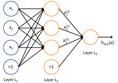
The most commonly used neural networks of direct distribution are designed for training with a teacher and are used, for example, for classification. An example of the topology of such a neural network is shown in the figure:


')
Training of such a neural network is usually done by back-propagating the error in such a way as to minimize the root-mean-square error of the network response on the training set. Thus, the training sample contains pairs of feature vectors (input data) and reference vectors (tagged data) {(x, y)} .

Now imagine that we have no tagged data — only a set of feature vectors {x} . The autoencoder is an unsupervised learning algorithm that uses a neural network and an error back-propagation method to ensure that the input feature vector triggers a network response equal to the input vector, i.e. y = x . Example of autoencoder:



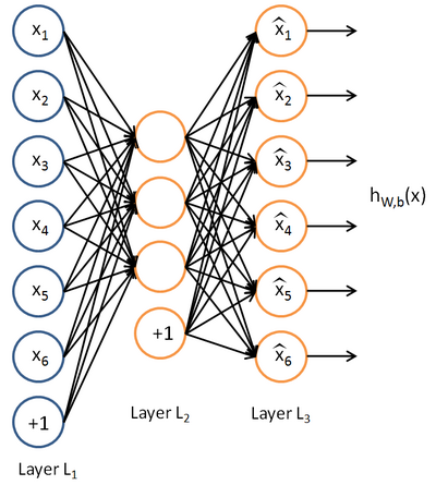
The autoencoder is trying to build a function h (x) = x . In other words, it tries to find an approximation of such a function so that the response of the neural network approximately equals the value of the input features. In order for the solution of this problem to be non-trivial, special conditions are imposed on the network topology:

• The number of neurons in the hidden layer must be less than the dimension of the input data (as in the figure), or
• Activation of neurons in the hidden layer must be sparse.

The first limitation allows you to get data compression when transmitting the input signal to the network output. For example, if the input vector is a set of image brightness levels of 10x10 pixels (100 signs total), and the number of neurons in the hidden layer 50, the network is forced to learn how to compress the image. Indeed, the requirement h (x) = x means that, based on the activation levels of fifty neurons of the hidden layer, the output layer must recover 100 pixels of the original image. Such compression is possible if there are hidden relationships in the data, a correlation of features, and in general some kind of structure. In this form, the operation of the auto-encoder is very similar to the method of principal component analysis (PCA) in the sense that the dimension of the input data decreases.

The second limitation - the requirement of sparse activation of neurons of the hidden layer - allows you to get non-trivial results even when the number of neurons of the hidden layer exceeds the dimension of the input data. If informality is described informally, then we will consider a neuron as active when the value of its transfer function is close to 1. If a sigmoid transfer function is used, but for an inactive neuron its value should be close to 0 (for the hyperbolic tangent function - to -1). Sparse activation is when the number of inactive neurons in the hidden layer significantly exceeds the number of active ones.

If we calculate the value of p as the average (according to the training sample) value of the activation of the neurons of the hidden layer, we can add an additional penalty term to the objective function used in the gradient training of the neural network by the method of backward error propagation. The formulas are in the original lectures, and the meaning of the penalty coefficient is similar to the regularization method for calculating the regression coefficients: the error function increases significantly if the value of p differs from the predetermined sparseness parameter. For example, we may require that the average activation value for a training sample be 0.05.

The requirement of sparse activation of neurons of the hidden layer has a bright biological analogy. Jeff Hawkins, author of the original theory of brain structure, notes the fundamental importance of inhibitory connections between neurons (see the Russian text Hierarchical Temporal Memory (HTM) and its cortical learning algorithms ). In the brain between neurons located in one layer there is a large number of "horizontal connections". Although neurons in the cerebral cortex are very tightly interconnected, numerous inhibitory (inhibitory) neurons ensure that only a small percentage of all neurons are active at a time. That is, it turns out that information is always presented in the brain only by a small number of active neurons from all those present there. This, apparently, allows the brain to make generalizations, for example, to perceive the image of a car from any angle just like a car.

Visualization of hidden layer functions

By training an autoencoder on an unmarked data set, you can try to visualize the functions approximated by this algorithm. Very visual is the visualization of the above example of teaching an encoder on images of 10x10 pixels. Let us ask ourselves the question: “What combination of input x will cause the maximum activation of the hidden neuron number i?” That is, what set of input data does each of the hidden neurons search for?

A nontrivial answer to this question is contained in the lecture , and we will limit ourselves to an illustration, which was obtained by visualizing the function of a network with a hidden layer of 100 neurons.



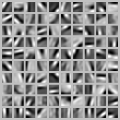
Each square fragment represents the input image x, which maximally activates one of the hidden neurons. Since the corresponding neural network was trained on examples of natural images (for example, fragments of photographs of nature), the neurons of the hidden layer independently studied the functions of detecting contours from different angles!

In my opinion, this is a very impressive result. The neural network itself, by observing a large number of various images, built a structure similar to the biological structures in the brain of humans and animals. As can be seen from the following illustration from the great book “From the Neuron to the Brain” by J. Nichols and others, this is how the lower visual divisions of the brain are arranged:



The figure shows the responses of complex cells in the cat's striped bark to visual stimuli. The cell responds best (most output pulses) to the vertical border (see the first fragment). The reaction to the horizontal border is practically absent (see the third fragment). A complex cell in a striped cortex approximately corresponds to our trained neuron in a hidden layer of an artificial neural network.

The whole set of neurons in the hidden layer has learned to detect contours (brightness difference boundaries) from different angles - just like in the biological brain. The following illustration from the book “From Neuron to Brain” schematically shows the axes of orientation of the receptive fields of neurons as they sink deeper into the cat's brain cortex. Similar experiments helped to establish that cells with similar properties in cats and monkeys are arranged in the form of columns running at certain angles to the surface of the cortex. Individual neurons in the column are activated by visual stimulation of the corresponding part of the field of view of the animal with a black stripe against a white background, rotated at a certain angle specific for each neuron in the column.

Self study

The most effective way to get a reliable machine learning system is to provide the learning algorithm with as much data as possible. According to the experience of solving large-scale tasks, there is a qualitative transition when the size of the training sample exceeds 1-10 million samples. You can try to get more tagged data for training with the teacher, but this is not always possible (and cost-effective). Therefore, the use of unmarked data for self-learning of neural networks seems promising.

Unmarked data contains less training information than tagged data. But the amount of data available for teaching without a teacher is much more. For example, an unlimited number of digital photographs are available on the Internet in image recognition tasks, and only a tiny percentage of them are marked.

In self-learning algorithms, we will give our neural network a large amount of unmarked data, from which the network will learn to extract useful signs. Further, these features can be used to train specific classifiers using relatively small labeled training samples.

We draw the first stage of self-learning in the form of a neural network with 6 inputs and three neurons of the hidden layer. The outputs of these neurons will be generalized signs that are extracted from the unmarked data by the sparse autoencoder algorithm.

Now you can train the output layer of the neural network, or use logistic regression, the support vector machine or the softmax algorithm for classifying training based on the identified features a. The input to these traditional algorithms will be the labeled training sample xm . There are two options for the self-learning network topology:

• To the input of a traditional classifier (for example, the output layer of a neural network) only signs a are fed;
• Signs a and input signs xm are fed to the input of the traditional classifier (for example, the output layer of the neural network).

Further in the Ng lectures, multilayer networks and the use of autoencoders for their training are considered.