Fractal Synthesis: IFS and L-systems

Introduction

[one]
A fractal (lat. "Fractus" - crushed, broken, broken) is called a complex geometric figure with the property of self-similarity, i.e. composed of several parts, each of which is similar to the whole figure. In a broader sense, fractals are understood as sets of points in Euclidean space that have an intermediate (fractional) metric dimension (Hausdorff dimension).
The Hausdorff dimension is a natural way to determine the dimension of a set in a metric space. The Hausdorff dimension agrees with our usual notions of dimension in those cases when these usual notions exist. For example, in a three-dimensional Euclidean space, the Hausdorff dimension of a finite set is zero, the dimension of a smooth curve is one, the dimension of a smooth surface is two, and the dimension of a set of nonzero volume is three.

Fractals are of several types:

• Geometric fractals are the most visible class of fractals. In two-dimensional space, they are obtained using a certain broken line (or surface in three-dimensional space), called a generator. In one step of the algorithm, each of the segments that make up the lo-manu is replaced by a generator-broken line at the appropriate scale. As a result of the infinite repetition of this procedure, a geometric fractal is obtained.
• Algebraic fractals are the largest group of fractals. Get them with the help of nonlinear processes in n-dimensional spaces. The most studied two-dimensional processes. Interpreting a nonlinear iterative process as a discrete dynamic system, one can use the terminology of the theory of these systems: phase portrait, steady state, attractor, etc. It is known that nonlinear dynamical systems possess several stable states. The state in which the dynamic system finds itself after a certain number of iterations depends on its initial state. Therefore, each steady state (or, as they say, an attractor) has a certain region of initial states, from which the system necessarily falls into the final states under consideration. Thus, the phase space of the system is divided into regions of attraction of attractors. If the phase is a two-dimensional space, then by coloring the areas of attraction with different colors, you can get a color phase portrait of this system (iterative process). Changing the color selection algorithm, you can get complex fractal paintings with fancy multi-color patterns. Surprise for mathematicians was the possibility of using primitive algorithms to generate very complex non-trivial structures.
• Stochastic fractals are another well-known class of fractals, which are obtained if in the iterative process you randomly change any of its parameters. At the same time, objects are very similar to natural ones - asymmetrical trees, indented coastlines, etc. Two-dimensional stochastic fractals are used in modeling the terrain and surface of the sea.

In addition to these, there are also:

• Handmade Fractals
• Natural fractals
• Deterministic fractals
• Nondeterministic fractals

Within the framework of this article, the methods of generating these fractals will be considered: L-systems and systems of iterated functions.

1. Systems of iterated functions

Traditionally in mathematics, spaces and sets contain points. However, there are spaces in which “points” are sets themselves. From a mathematical point of view, the advantage of abstraction from a point is to achieve commonality.
An example of this is contraction mappings and related convergence theorems. Compressing mappings are defined in metric spaces as mappings reducing the distance between points. Contractive mappings have an important property. If we take any point and begin to apply the same contraction mapping to it iteratively: f (f (f ... f (x))), then the result will always be the same point. The more times we apply, the more precisely we will find this point. It is called a fixed point and for each compressing map it exists, and only one. Iterated Function Systems (IFS) are an example of the application of this theory.

1.1 Definition

The system of iterated functions is a finite set of functions Fi: X -> X in a metric space X. Each of them expands to a map Fi: H (X) -> H (X), where H (X) is the space of which points are non-empty compressed subsets of X. If we use the Hausdorff metric, then H (X) is complete if X was complete. In addition, the compression FiX X remain compression on H (X). In the aggregate, {Fi} defines a new compression F: H (X) -> H (X), according to the following formula: for each A∈H (X), F (A) = ∪Fi (A). From the general theory, for a complete metric space X, F has a fixed point AF: F (AF) = AF, which can be achieved by successive approximations from any starting point. Fixed IFS points are sometimes called attractors or invariants.

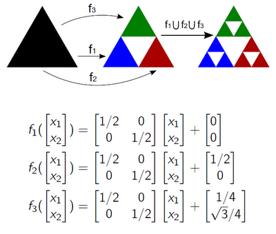
Figure 6. An example of building a Sierpinski triangle using IFS.
Thus, two problems arise. The first is to find an attractor given by IFS. The second problem is the opposite of the first: for a given set A∈H (X), find IFS {Fi} for which A is an attractor.

1.2 Deterministic algorithm

The first problem is solved using a deterministic algorithm.
Let's start with the set A0∈H (X) and let's sequentially calculate
Ak = ∪Fi (Ak-1) = F (Ak-1), k> 1. The series {Ak) converges to the attractor AF with k.

1.3 Algorithm of random iterations

The mathematics of an alternative algorithm — a random iteration algorithm — is more complicated, but its application is simpler. We compare the positive frequencies pi to the mappings Fi. We start at an arbitrary point x0∈X. At each step k + 1, choose xk + 1 from the set {Fi (xk)}. Fj (xk) is chosen with probability pj / pi. The sequence [5] {xk} converges to AF. In practice, in order to display the AF approximation on a computer, the sequence points are displayed on the screen. The numbers {pi} do not change AF in any way, but they significantly influence the process of displaying its approximations.

1.4 Collage Theorem

The inverse problem is approximately solved by the collage theorem. Quoting M. Barnsley: “The theorem says that in order to find an IFS attractor that is“ similar ”to this set, it is necessary to find a set of compressing mappings of some larger set including its subset of the original set, such that the union, or collage, of the set of this set is approximated would be the original set.

1.5 Use

[2]
The main scope of IFS is image compression. Arbitrary images, unlike fractals, are not self-similar, so this problem is not solved so easily. How to do it came up with in 1992, Arnold Zhakin, at that time - Michael Barnsley's graduate student.
Self-similarity is necessary - otherwise affine transformations that are limited in their capabilities will not be able to bring images closer. And if it is not between the part and the whole, then you can search between the part and the part.
The simplified coding scheme looks like this:

• The image is divided into small non-overlapping square areas, called rank blocks.
• A pool of all possible overlapping blocks is built four times as large as a range of domain blocks.
• For each rank block, we “try on” the domain blocks in turn and look for such a transformation that makes the domain block most similar to the current rank-and-go.
• The pair “transformation - domain block”, which is close to the ideal, is assigned to the rank block. Transformation coefficients and domain block coordinates are saved to the encoded image. We don’t need the contents of the domain block - you remember, we don’t care from which point to start.

In the picture, the rank block is marked in yellow, the corresponding domain is marked in red. Also shown are the conversion steps and the result.

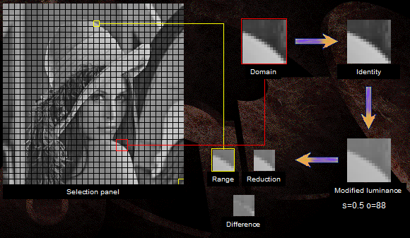
Figure 7. An example of image compression.
Obtaining an optimal transformation is a separate topic, but it is not a big deal. But another drawback of the scheme is visible to the naked eye. The two-megapixel image will contain a huge number of 32x32 domain blocks. Their exhaustive search for each rank block is the main problem of this type of compression - coding takes a lot of time. They are struggling with this using various tricks, such as narrowing the search area or pre-classifying domain blocks.

Decoding is done simply and fairly quickly. We take any image, divide it into ranking areas, and successively replace them with the result of applying the corresponding transformation to the corresponding domain area (whatever it may contain at the given moment). After several iterations, the original image will look like itself:

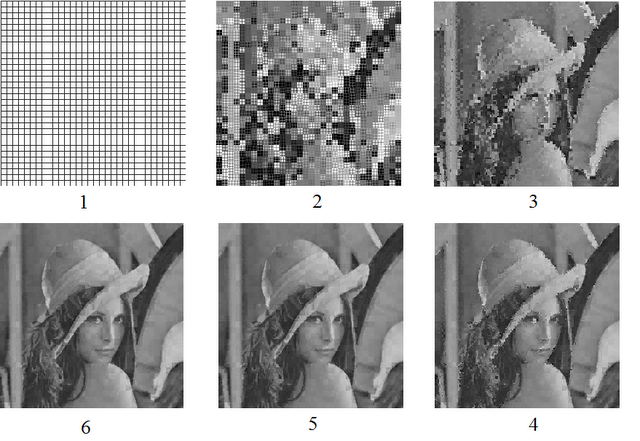
Figure 8. Example of restoring a compressed image.
')

2. Lindenmayer Systems

[3]
The beauty of plants has attracted the attention of mathematicians for centuries. The interesting geometric properties of plants, such as the symmetry of the leaves relative to the central axis, the radial symmetry of flowers, and the spiral arrangement of seeds in the cones, have been studied most actively. “Beauty is associated with symmetry” (H. Weyl. Symmetry). During the growth of living organisms, especially plants, one can clearly see regularly repeated multicellular structures. In the case of compound leaves, for example, small leaves, which are part of a large adult leaf, have the same shape that the whole leaf had at an early stage of formation.

In 1968 Hungarian biologist and botanist Aristid Lindenmayer (Aristid Lindenmayer) proposed a mathematical model to study the development of simple multicellular organisms, which was later expanded and used to model complex branching structures - various trees and flowers. This model is called the Lindenmayer System, or simply the L-System.

2.1 Basic ideas

The main idea of ​​L-systems is the constant rewriting (rewriting) of line elements. What is it about? In this case, rewriting is a method of obtaining complex objects by replacing parts of a simple initial object according to certain rules. A classic example is Koch's dream. In the figure, the initiator is the initial object, the faces of which are replaced by the generator object. Next, the same thing is done with the new object.

Figure 1. Koch snowflake.

Returning to L-systems and drawing an analogy with fractals, we can say that the L-system operates on a string of characters according to special rules, starting with the original simple axiom. Thus, the L-system is a mathematical grammar. But the fundamental difference between L-systems and formal grammars is that the rules apply simultaneously to the entire line, to each character, plus, there are no concepts of terminal and non-terminal characters. That is, the "conclusion" of this grammar can continue indefinitely.
The following picture shows the relationship between context-free (OL), context-dependent (IL) L-systems and other formal grammars in the Chomsky hierarchy.

Figure 2. Chomsky's hierarchy.

2.2 Simplest L-systems

Also, as in Chomsky’s classification, L-systems have their own classification from simple to complex and powerful.
The simplest example is deterministic context-free L-systems or abbreviated DOL. I don’t like formal grammar definitions, so I’ll just say it in my own words. There is a set of symbols - the alphabet. This alphabet records the string with which the L-system works. There is an axiom - the original string of one or more letters and a set of rules of the form a → ab. During each iteration of the algorithm, applying a rule to a letter from the current line, it (the letter) is replaced with a set of letters to the right of the arrow. It is easier to consider a specific example of the development of the multicellular organism Anabaena catenula, which Lindenmeier studied when he proposed the model of L-systems.
Let our alphabet consist of the following characters, each of which denotes a certain cell: alar bl br.
Axiom consists of one symbol:
ω: ar
And the four rules.
p1: ar → albr
p2: al → blar
p3: br → ar
p4: bl → al

The rules say which symbols change to which in the process of growth of the organism. The picture shows how, applying the rules, we observe the “cell division” and development.

Figure 3. L-system simulating the development of Anabaena catenula.

2.4 Using LOGO

So far we have seen how to draw a one-dimensional bacterium, but using the well-known children's programming language LOGO, in which it is proposed to control the turtle and draw figures on the screen, one can already draw two-dimensional and three-dimensional fractals and repeating structures. How? It's simple. Take the alphabet, in which each character means a certain command for a two-dimensional or three-dimensional bug:

• F - move forward and draw a line
• f - go ahead without drawing anything
• + - turn left
• - - turn right
• & - turn down
• ^ - turn up
• \ - lean to the left
• / - lean to the right
• | - turn 180 degrees

These commands use the standard values ​​of the rotation angle δ, the step length and the basis vectors of the two-dimensional and three-dimensional space. Examples of two-dimensional fractals and L-systems generating them can be seen in the following picture:

Figure 4. Examples of L-systems.

2.5 Plants and Branching Structures

Everything that was before is, in general, continuous curves. Such a modeling method is not suitable for modeling plants with their branching topology. To do this, alpha-vit characters [and] were added, which indicate the beginning and end of branching, respectively. When the turtle encounters the symbol [, its current state is written to the stack and retrieved from there when the symbol is encountered]. Already such a simple grammar can generate quite interesting two-dimensional and three-dimensional objects similar to trees.

Figure 5. Examples of branching L-systems.

2.6 Stochastic L-systems

Stochastic L-systems add the ability to specify the probability of the fulfillment of a rule, and in the general case are not deterministic, because different rules may have the same symbol to the left. This introduces some element of randomness into the resulting structures.

2.7 Context-sensitive L-systems

As well as contextual dependence in formal grammars, in the L-system, the syntax of rules is complicated and takes into account the environment of the replaced character.

2.8 Parametric L-systems

A variable variable (possibly more than one) is added to each symbol, which allows, for example, specifying the rotation angle for + and -, the stride length and line thickness, checking the conditions for applying the rule, counting the number of iterations and sending “signals” back and forth . An example of a parametric L-system.

ω: B (2) A (4, 4)
p1: A (x, y): y <= 3 → A (x ∗ 2, x + y)
p2: A (x, y): y> 3 → B (x) A (x / y, 0)
p3: B (x): x <1 → C
p4: B (x): x> = 1 → B (x - 1)

Parametric context-dependent L-systems make it possible to simulate the growth of multicellular organisms and plants, taking into account biochemical processes and the environment.

2.9 Usage

Back in the late 80s, L-systems were used to visualize plant models. Now the possibilities of computers are far ahead. Many games and 3d modeling tools use procedural content generation, including L-systems. As you can see, from a set of simple rules you can get a huge number of different plants and plant whole fields with them.