And again about sorting: choose the best algorithm
Recently, at Habré, another one raised the topic of sorting algorithms, namely, the Timsort method was well described.
He, having a complexity of no more than O (n log n), is accelerated in the case of sorting partially ordered data and has a complexity of O (n) if the data is initially sorted. But this is not the only algorithm with such declared properties. There are at least two more or less well-known methods with similar complexity - these are Smoothsort and Shell sorting.
But the fact that they have a similar complexity does not mean at all that they all work equally fast. I tried to compare their actual performance on different data and see who is better at their task.
')
Usually, the real time of operation of different algorithms with the same complexity on the same data may differ several times. Let's remember why this happens and ask Wikipedia what the phrase “the algorithm has O (n log n) complexity” means
And this coefficient C influences the real time of the agitourt operation. The more complex the algorithm, the more advanced the data structures used in it, the greater the number of operations that must be performed during the execution of the program to support all the necessary variables and structures. That is, the greater the coefficient C and the real time of work. Of course, this coefficient also depends on the specific implementation, but if you pay attention to the code you write and know the features of the development language, the main contribution to this constant will be made by the algorithm.
Therefore, it was interesting to see what real performance gain each of these algorithms gives in the case of partially ordered data, and how significant this gain, if any, is. For this, several experiments were carried out. But for starters, I want, without going into details, to remind how the above-mentioned algorithms work. If anyone is not interested, please immediately compare.
Good description here , just to quote the main idea:
The complexity at best (the input data is sorted in any order, maybe even the opposite required) is O (n), and in general is not worse than O (n log n).
O (n) extra memory required.
The big advantage is that the algorithm is a combination of other fairly simple algorithms, therefore it does not require sophisticated operations with different data structures. Therefore, good performance is expected.
It was invented by the notorious E. V. Deikstroy in 1981 and is a development of the idea of Heapsort - sorting using the binary heap (well, or a pyramid, as you like).
To begin, let me remind you how Heapsort works:
There is an optimization that allows you to perform the first step with O (n) complexity, but the second step will still have O (n log n) complexity.
The algorithm requires O (1) additional memory, the heap is stored directly in the original data array.
Dijkstra proposed replacing one binary heap in the algorithm with an ordered set of Leonardo heaps, which are based on special Leonardo numbers.
Leonardo numbers are defined recurrently as follows:
Leonardo's k-th heap is a binary tree with the number of vertices L (k) satisfying the following conditions:
Heaps should be ordered by size (the largest - from the left), and the values of their roots should be non-decreasing from left to right, from which it follows that the maximum element of the structure will always be the root of the right-most heap. The structure is stored in the source array, the size of the additional memory is O (1).
Any natural number can be decomposed into a sum of Leonardo numbers, which means that the structure described above can be constructed for any number of numbers.

An example of the structure of Leonardo heaps for 13 elements. Three heaps are used: 4th, 2nd and 1st.
To add an element to such a structure, it is necessary to rebuild some of the heaps so that the sum of their sizes becomes equal to the new number of elements, and also to make sure that the roots of the heaps remain ordered in ascending order. Such an operation has a complexity of no more than O (log n).

When adding an item, you need to rebuild the heaps (Property of 1 Leonardo heap in the picture is not restored)
Extracting the maximum is similar to adding an element and also has a complexity of no more than O (log n).
The Smoothsort sorting algorithm itself works in two stages, like Heapsort:
The advantage of using such a structure is that in the case of an already sorted input sequence, heap operations and extraction of all elements will have total complexity O (n). And it is argued that as the degree of ordering of the data to be sorted decreases, the complexity will smoothly (smoothly) increase from O (n) to O (n log n). Hence the name - Smoothsort.
In general, the algorithm is far from trivial, and in addition is not very clearly described. Materials:
Wikipedia article
The original article is incomprehensible, you have to understand for a long time.
The original article, commented on by Hartwig Thomas , is the same, but a normal font + explanatory comments. But it doesn't get any easier :)
The study of the algorithm from K. Schwarz is already clearer, but some significant optimizations are not described at all. Illustrations inserted from there.
Shell sorting is a superstructure above sorting inserts; instead of one passage, we make several, and on the i-th passage, we sort the subarrays of elements standing apart from each other at a distance d i .
In this case, on the last pass, d i must be equal to 1 (that is, the last step is the usual sorting by inserts), this guarantees the correctness of the algorithm.
For example: let it be necessary to sort an array of 12 elements, the number of passes is 3, d 1 = 5, d 2 = 3, d 3 = 1
In the first step, the following arrays will be sorted:
On the second:
And on the third array (a1, ..., a12) entirely
The advantage over the usual sorting by inserts is that in the first passes the array elements move not in steps 1, but in d i , but by the last pass some locality has already been reached (the elements are close to their final places), so there is no need to produce a large amount exchanges.
The complexity of the algorithm depends on the choice of the number of passes and d i values, and can vary greatly; Wikipedia has a special table. For testing, I chose the option described here , in the worst case, its complexity is O (n 4/3 ), and on average O (n 7/6 ).
If the data is initially sorted in the right order, then no exchange will be made, all passes will pass “to idle”. Therefore, the complexity in this case depends only on the number of passes. If their number is fixed, then it will be just O (n).
O (1) additional memory required.
You can read more here , here and here .
Actually, here's the most interesting part - to test all the above methods on different data and compare their real time.
The following implementations took part in the testing, all code is written in pure C:
Only the response time of the sorting algorithm (in seconds) was measured, the generation time of the test data was not taken into account. Each algorithm was run on the same data three times, the best result was taken into account (so that the short-term system loads do not affect our honest experiment :))
Iron: HP dv3510er laptop, Intel Core 2 Duo 2GHz, 2GB RAM.
OS: Ubuntu 11.10
Four experiments were performed on various data:
The objective of this experiment is to compare the performance of algorithms on arbitrary, in no way ordered data. 10 sets of 10 8 random natural numbers were generated, the average operation time was measured for each algorithm.
The complexity of all tested algorithms in the case of arbitrary data is equal (except for ShellSort) O (n log n). Actually, here you can trace the influence of the very constant C.

As we can see, the algorithms that do not use any data structures have pretty seriously gone ahead. Further we will consider partially ordered data.
Given 10 8 different natural numbers, sorted in ascending order. We group them by k consecutive elements and rearrange all the groups in the reverse order.
Example for ten numbers: 1 2 3 4 5 6 7 8 9 10
k = 1: 10 9 8 7 6 5 4 3 2 1
k = 3: 8 9 10 5 6 7 2 3 4 1
k = 5: 6 7 8 9 10 1 2 3 4 5
k = 10: 1 2 3 4 5 6 7 8 9 10
Groups are “independent” from each other in the sense that they do not intersect over the range of values stored in them. That is, elements of any group are larger than elements of all groups to the right, as well as less than those that are to the left.
Measurements were made for all k equal to powers of 10.
You may notice the following patterns:
10 8 integers are given from a limited range (in our case [0 ... 100000]) and they are ordered by groups of arbitrary size from 1 to k.
Such a data set already somehow corresponds to the data from real-world problems; I had to deal with those for calculating Dies proximity factors.

In this example, Smoothsort showed itself from the wrong side again, it works longer than Heapsort, and behaves the same way. Timsort is again ahead.
We will generate partially ordered data in another way: take 10 8 arbitrary natural numbers, sort them and make k arbitrary permutations of two elements in places.

And this experiment finally allows Smoothsort to “open up”: acceleration becomes noticeable with increasing degree of sorting of input data. This is due to the fact that, unlike previous experiments, here the algorithm “moves” along Leonardo’s heaps only a very small fixed number of elements, which does not entail a large number of operations to move elements inside the heaps. But after a certain point, he again becomes too "long."
As you can see, the practical benefits of the described algorithms are there, they cope with their task with varying success. Timsort became the absolute leader - giving a noticeable acceleration with increasing degree of data ordering and working at the Quicksort level in normal cases. No wonder it is recognized and embedded in Python, OpenJDK and Android JDK.
There is quite a bit of information about Smoothsort on the network (compared to other algorithms), and not surprisingly: because of the complexity of the idea and the controversial performance, it is rather an algorithmic sophistication than an applicable method. I found only one real application of this algorithm - in the sofia-sip library, intended for building IM and VoIP applications.
The appearance of Shellsort in this test is a rather controversial point, because its asymptotic complexity is somewhat greater than that of the other two algorithms. But it has two big advantages: the simplicity of the idea and the algorithm that almost always avoids Smoothsort in terms of speed and simplicity of implementation - working code takes only a few dozen lines, while good implementations of Timsort and Smoothsort require more than a hundred lines.
I want to note that I compared exactly the performance, and did not specifically focus on other parameters (such as using additional memory).
My subjective conclusion is that if you need a very good sorting algorithm for embedding in a library or a large project, then Timsort is best suited. In the case of small tasks, where there is no time and the need to write complex algorithms, and the result is needed quickly, Quicksort can be easily dispensed with - as it gives the best performance that is simple in writing algorithms.
Thanks for reading. I hope you were interested.
He, having a complexity of no more than O (n log n), is accelerated in the case of sorting partially ordered data and has a complexity of O (n) if the data is initially sorted. But this is not the only algorithm with such declared properties. There are at least two more or less well-known methods with similar complexity - these are Smoothsort and Shell sorting.
But the fact that they have a similar complexity does not mean at all that they all work equally fast. I tried to compare their actual performance on different data and see who is better at their task.
')
Usually, the real time of operation of different algorithms with the same complexity on the same data may differ several times. Let's remember why this happens and ask Wikipedia what the phrase “the algorithm has O (n log n) complexity” means
The complexity of the algorithm O (n log n) means that for large n the running time of the algorithm (or the total number of operations) is no more than C · n log n, where C is some positive constant.
And this coefficient C influences the real time of the agitourt operation. The more complex the algorithm, the more advanced the data structures used in it, the greater the number of operations that must be performed during the execution of the program to support all the necessary variables and structures. That is, the greater the coefficient C and the real time of work. Of course, this coefficient also depends on the specific implementation, but if you pay attention to the code you write and know the features of the development language, the main contribution to this constant will be made by the algorithm.
Therefore, it was interesting to see what real performance gain each of these algorithms gives in the case of partially ordered data, and how significant this gain, if any, is. For this, several experiments were carried out. But for starters, I want, without going into details, to remind how the above-mentioned algorithms work. If anyone is not interested, please immediately compare.
Compare Algorithms
Timsort
Good description here , just to quote the main idea:
- A special algorithm splits the input array into subarrays.
- Each subarray is sorted by normal sorting by inserts.
- Sorted subarrays are assembled into a single array using modified merge sorting.
The complexity at best (the input data is sorted in any order, maybe even the opposite required) is O (n), and in general is not worse than O (n log n).
O (n) extra memory required.
The big advantage is that the algorithm is a combination of other fairly simple algorithms, therefore it does not require sophisticated operations with different data structures. Therefore, good performance is expected.
Smoothsort
It was invented by the notorious E. V. Deikstroy in 1981 and is a development of the idea of Heapsort - sorting using the binary heap (well, or a pyramid, as you like).
To begin, let me remind you how Heapsort works:
- Build a heap by adding one element to it (complexity O (log n) for each, total O (n log n))
- Extract the maximum element that lies in the root of the heap, until it becomes empty. Since when a root is removed, the heap splits into two independent ones, it is required to collect them into one by O (log n). In total for n elements - also O (n log n)
There is an optimization that allows you to perform the first step with O (n) complexity, but the second step will still have O (n log n) complexity.
The algorithm requires O (1) additional memory, the heap is stored directly in the original data array.
Dijkstra proposed replacing one binary heap in the algorithm with an ordered set of Leonardo heaps, which are based on special Leonardo numbers.
Leonardo numbers are defined recurrently as follows:
Here are the first few members of this sequence:L (0) = 1, L (1) = 1, L (i) = L (i - 2) + L (i - 1) + 1
1, 3, 5, 9, 15, 25, 41, ...
Leonardo's k-th heap is a binary tree with the number of vertices L (k) satisfying the following conditions:
- The number written in the root is not less than the numbers in the subtrees (and therefore a lot)
- The left subtree is (k-1) -I Leonardo heap
- Right - (k-2) -I
Heaps should be ordered by size (the largest - from the left), and the values of their roots should be non-decreasing from left to right, from which it follows that the maximum element of the structure will always be the root of the right-most heap. The structure is stored in the source array, the size of the additional memory is O (1).
Any natural number can be decomposed into a sum of Leonardo numbers, which means that the structure described above can be constructed for any number of numbers.
An example of the structure of Leonardo heaps for 13 elements. Three heaps are used: 4th, 2nd and 1st.
To add an element to such a structure, it is necessary to rebuild some of the heaps so that the sum of their sizes becomes equal to the new number of elements, and also to make sure that the roots of the heaps remain ordered in ascending order. Such an operation has a complexity of no more than O (log n).
When adding an item, you need to rebuild the heaps (Property of 1 Leonardo heap in the picture is not restored)
Extracting the maximum is similar to adding an element and also has a complexity of no more than O (log n).
The Smoothsort sorting algorithm itself works in two stages, like Heapsort:
- Adding one by one, a lot of Leonardo heaps are built for all elements (no more than O (log n) per each)
- Maximum elements are extracted from the constructed structure in turn (the root of the rightmost heap is always the maximum) and the structure is restored as necessary (no more than O (log n) per element)
The advantage of using such a structure is that in the case of an already sorted input sequence, heap operations and extraction of all elements will have total complexity O (n). And it is argued that as the degree of ordering of the data to be sorted decreases, the complexity will smoothly (smoothly) increase from O (n) to O (n log n). Hence the name - Smoothsort.
In general, the algorithm is far from trivial, and in addition is not very clearly described. Materials:
Wikipedia article
The original article is incomprehensible, you have to understand for a long time.
The original article, commented on by Hartwig Thomas , is the same, but a normal font + explanatory comments. But it doesn't get any easier :)
The study of the algorithm from K. Schwarz is already clearer, but some significant optimizations are not described at all. Illustrations inserted from there.
Shellsort (Sort Shell)
Shell sorting is a superstructure above sorting inserts; instead of one passage, we make several, and on the i-th passage, we sort the subarrays of elements standing apart from each other at a distance d i .
In this case, on the last pass, d i must be equal to 1 (that is, the last step is the usual sorting by inserts), this guarantees the correctness of the algorithm.
For example: let it be necessary to sort an array of 12 elements, the number of passes is 3, d 1 = 5, d 2 = 3, d 3 = 1
In the first step, the following arrays will be sorted:
(a1, a6, a11), (a2, a7, a12), (a3, a8), (a4, a9), (a5, a10)
On the second:
(a1, a4, a7, a10), (a2, a5, a8, a11), (a3, a6, a9, a12)
And on the third array (a1, ..., a12) entirely
The advantage over the usual sorting by inserts is that in the first passes the array elements move not in steps 1, but in d i , but by the last pass some locality has already been reached (the elements are close to their final places), so there is no need to produce a large amount exchanges.
The complexity of the algorithm depends on the choice of the number of passes and d i values, and can vary greatly; Wikipedia has a special table. For testing, I chose the option described here , in the worst case, its complexity is O (n 4/3 ), and on average O (n 7/6 ).
If the data is initially sorted in the right order, then no exchange will be made, all passes will pass “to idle”. Therefore, the complexity in this case depends only on the number of passes. If their number is fixed, then it will be just O (n).
O (1) additional memory required.
You can read more here , here and here .
Comparison
Actually, here's the most interesting part - to test all the above methods on different data and compare their real time.
The following implementations took part in the testing, all code is written in pure C:
- TimSort - a David R. Maclver implementation written for his TimSort article - Good, Optimized Implementation
- SmoothSort is one of my implementations, the fastest that I managed to write
In general, writing this algorithm more or less effectively is not very easy. You can probably write faster and more optimally, but after four attempts I decided not to continue :) - ShellSort is an implementation based on an example from here.
- Also, the usual quicksort and heapsort recursive implementations were added to the comparison in order to be able to evaluate the advantages of the considered methods over the traditional
Test parameters
Only the response time of the sorting algorithm (in seconds) was measured, the generation time of the test data was not taken into account. Each algorithm was run on the same data three times, the best result was taken into account (so that the short-term system loads do not affect our honest experiment :))
Iron: HP dv3510er laptop, Intel Core 2 Duo 2GHz, 2GB RAM.
OS: Ubuntu 11.10
Four experiments were performed on various data:
Experiment 1: Work on ordinary data
The objective of this experiment is to compare the performance of algorithms on arbitrary, in no way ordered data. 10 sets of 10 8 random natural numbers were generated, the average operation time was measured for each algorithm.
The complexity of all tested algorithms in the case of arbitrary data is equal (except for ShellSort) O (n log n). Actually, here you can trace the influence of the very constant C.
As we can see, the algorithms that do not use any data structures have pretty seriously gone ahead. Further we will consider partially ordered data.
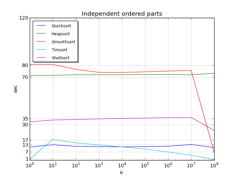
Experiment 2: Independent sorted groups of equal size
Given 10 8 different natural numbers, sorted in ascending order. We group them by k consecutive elements and rearrange all the groups in the reverse order.
Example for ten numbers: 1 2 3 4 5 6 7 8 9 10
k = 1: 10 9 8 7 6 5 4 3 2 1
k = 3: 8 9 10 5 6 7 2 3 4 1
k = 5: 6 7 8 9 10 1 2 3 4 5
k = 10: 1 2 3 4 5 6 7 8 9 10
Groups are “independent” from each other in the sense that they do not intersect over the range of values stored in them. That is, elements of any group are larger than elements of all groups to the right, as well as less than those that are to the left.
Measurements were made for all k equal to powers of 10.
You may notice the following patterns:
- Quicksort and Heapsort also love it when the data is partially sorted (compare both graphs). It does not affect the asymptotic complexity, but the speed of work still increases several times
- Timsort doesn't care in which order the data is sorted, in both cases it works very fast
- Smoothsort has its own understanding of partial data ordering. The real performance gain in this test is noticeable only with fully sorted data. Even in the case when the array is a small amount of completely sorted pieces, in order to rearrange them in places, the algorithm needs to perform a huge number of operations with heaps of Leonardo, which are rather “heavy”
- Shellsort, despite the greater complexity (with n = 10 8 n 7/6 > n log n), often works in less time than Smoothsort. This is due to the relative simplicity of the algorithm. But with fully sorted data, Shellsort is still forced to make all the passes, even if not rearranging a single element. Therefore, for k = 10 8, the result is almost the worst of the algorithms considered.
Experiment 3: Sorted groups of different sizes, limited range of values
10 8 integers are given from a limited range (in our case [0 ... 100000]) and they are ordered by groups of arbitrary size from 1 to k.
Such a data set already somehow corresponds to the data from real-world problems; I had to deal with those for calculating Dies proximity factors.
In this example, Smoothsort showed itself from the wrong side again, it works longer than Heapsort, and behaves the same way. Timsort is again ahead.
Experiment 4: Arbitrary Permutations
We will generate partially ordered data in another way: take 10 8 arbitrary natural numbers, sort them and make k arbitrary permutations of two elements in places.
And this experiment finally allows Smoothsort to “open up”: acceleration becomes noticeable with increasing degree of sorting of input data. This is due to the fact that, unlike previous experiments, here the algorithm “moves” along Leonardo’s heaps only a very small fixed number of elements, which does not entail a large number of operations to move elements inside the heaps. But after a certain point, he again becomes too "long."
Results
As you can see, the practical benefits of the described algorithms are there, they cope with their task with varying success. Timsort became the absolute leader - giving a noticeable acceleration with increasing degree of data ordering and working at the Quicksort level in normal cases. No wonder it is recognized and embedded in Python, OpenJDK and Android JDK.
There is quite a bit of information about Smoothsort on the network (compared to other algorithms), and not surprisingly: because of the complexity of the idea and the controversial performance, it is rather an algorithmic sophistication than an applicable method. I found only one real application of this algorithm - in the sofia-sip library, intended for building IM and VoIP applications.
The appearance of Shellsort in this test is a rather controversial point, because its asymptotic complexity is somewhat greater than that of the other two algorithms. But it has two big advantages: the simplicity of the idea and the algorithm that almost always avoids Smoothsort in terms of speed and simplicity of implementation - working code takes only a few dozen lines, while good implementations of Timsort and Smoothsort require more than a hundred lines.
I want to note that I compared exactly the performance, and did not specifically focus on other parameters (such as using additional memory).
My subjective conclusion is that if you need a very good sorting algorithm for embedding in a library or a large project, then Timsort is best suited. In the case of small tasks, where there is no time and the need to write complex algorithms, and the result is needed quickly, Quicksort can be easily dispensed with - as it gives the best performance that is simple in writing algorithms.
Thanks for reading. I hope you were interested.
Source: https://habr.com/ru/post/133996/
All Articles