Upgrade viola jones
In my previous topic, I tried to show how the Viola Jones method works, using what technologies and internal algorithms. In this post, in order not to interrupt the chain, there will also be a lot of theory, it will be shown at the expense of what can be improved and so beautiful method. If we also describe the software implementation here , then there will be a huge canvas that will be very inconvenient to read, and it will not look at all - it was decided to divide the amount of information into two separate posts. Below is a theory, few pictures, but many useful things.
The person does not even notice how he simply copes with the tasks of detecting faces and emotions with the help of his vision. When the eye looks at the surrounding faces of people, objects, nature, one does not subconsciously feel how much work the brain does to process the entire flow of visual information. It will not be difficult for a person to find a familiar person in a photograph, or to distinguish a snide grimassu from a smile.
A person tries to recreate and build a computer system for detecting faces and emotions - he partly succeeds in this, but every time he has to face big problems in recognition. Computers nowadays can easily store huge amounts of information, pictures, video and audio files. But to find computing systems with the same ease, for example, the right photo with a certain emotion of the right person from your own personal photo gallery is a difficult task. The solution of this problem is hampered by some factors :
The list can be continued for a long time. But attention is focused on the most important points, so it makes no sense to list all the interfering parameters.
Comparison of the quality of recognition of various methods is complicated by many reasons. One of them, and the most significant one, is that in most cases you can only rely on test data provided by the authors themselves, since conducting large-scale research on the implementation of most known methods and comparing them to each other on a single set of images is not possible:
The main points influencing the choice of the method of solving the problem and the conditions of the criteria revealed the following (in the development process, those that are italicized are most optimal):
')
• restrictions on individuals:
- a limited, predetermined set of people;
- restrictions on the possible race of people or on the characteristic differences on the face (for example, facial hair, glasses);
- no restrictions .
• face position on the image:
- frontal;
- tilt at a known angle;
- any slope .
• image type:
- color;
- black and white;
- any .
• face scale:
- fully in the "main frame";
- localized in a certain place with a certain size;
- it doesn't matter .
• resolution and image quality:
- bad / bad;
- bad / good;
- only good;
- any .
• noise, interference, moire:
- weak;
- strong;
- it doesn't matter .
• number of faces in the image:
- known;
- approximately known;
- unknown .
• lighting:
- known;
- approximately known;
- any .
• background:
- fixed;
- contrast monophonic;
- low contrast noise;
- unknown;
- no difference .
• importance of research:
- it is more important to identify all faces and features ;
- to minimize the errors of false detections by minimizing the detections on the image.
The Viola-Jones method sometimes produces startling errors, as some Habrawers mentioned. Therefore, the most logical solution in this situation was to modify the Viola-Jones algorithm and improve its recognition characteristics, if at all possible.
The method proposed below suggests a possible disposal of:
Taking into account the above, this method of work should reduce the time for determining emotions.
The scheme of the new method is presented in the figure below:

So, to improve the capabilities of the algorithm and the quality of finding inclined facial features, I propose such a variant of new types of features, as in the figure.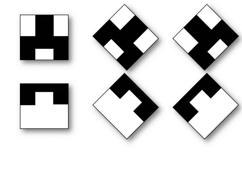 Such signs were not chosen by chance, but in connection with the silhouettes of the desired features. Using these features, the program will search much faster for the nose, eyebrows and mouth, but it will spend a little more time on other facial features than in the standard algorithm, but additional features should be implemented: in general, recognition milliseconds are won and slightly, but accuracy increases.
The described algorithms that the Viola-Jones method uses are quite widely used. The method itself can successfully interact with other algorithms and can be adapted to specific needs and requirements. Also, it works not only with static images, you can freely process data in real time. However, even he does not provide the perfect recognition of emotions. Let's try to raise the recognition percentage even higher with the help of Viola-Jones. For this purpose, in order to increase productivity, it was decided to perform image pre-processing .
To create a fast and reliable way to determine the likely areas of a person’s face in order to speed up processing at further stages of detection, an algorithm is proposed for determining and distinguishing boundary contours . The idea of this approach is that it is possible to emphasize the areas in which the person and his features are most likely to be found. Thus, not only is the acceleration of the algorithm achieved, but the probability of false detection of faces is also reduced. These steps will be illustrated in the original image:

First you need to translate the image in grayscale . For this purpose it is convenient to present the image in the color model YUV . For this conversion is performed:

The translated halftone image is smoothed and spatial differentiation is performed - the gradient of the intensity function at each point of the image is calculated. It is assumed that the regions correspond to real objects, or their parts, and the boundaries of regions correspond to the boundaries of real objects. Detection of brightness gaps using a sliding mask (sliding window) is used . In different textbooks and articles, it is variously called, usually referred to as a filter or a kernel, which is a square matrix corresponding to the mapped Y of the original image. The spatial filtering scheme is shown below:

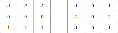
In the applied method, using special kernels, known as " Sobel operators ", operating in the image area of 3 * 3 size, weighting factor 2 is used for middle elements. The coefficients of the kernel are chosen so that when it is applied, the smoothing in one direction is simultaneously performed and the spatial derivative is calculated in the other. The masks used by the Sobel operator are shown below:
From them we get the components of the gradient G x and G y :
To calculate the magnitude of the gradient, these components must be used together:
 (1.4)
(1.4)
or (1.5)
(1.5)
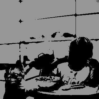
The result shows how "sharply" or "smoothly" the brightness of the image at each point changes, which means that the probability of finding a point on the face, as well as the orientation of the border. The result of the work of the Sobel operator at the point of the constant brightness region will be the zero vector, and at the point lying on the border of the regions of different brightness, the vector intersecting the boundary in the direction of increasing brightness. Also, the result of the work is the translation of the photo into boundary contours (this can be seen in the transformed picture):

Further, the same halftone image is subjected to a threshold classification (thresholding) , or the choice of the threshold in brightness. The meaning of this threshold is to separate the desired light object (foreground) and dark background (background), where the object is a collection of those pixels whose brightness exceeds the threshold (I> T), and the background is a collection of other pixels whose brightness is lower threshold (I <T). An approximate algorithm for working with the global threshold in automatic mode looks like this:

The Sobel operator cannot do this, since it gives a lot of noise and interference, therefore the halftone image must be binarized . There are dozens of methods for selecting the threshold, but it is the method that was invented by the Japanese scientist Nobuyuki Otsu (Otsu's Method) in 1979 [1], because he is fast and efficient. The brightness values of the image pixels can be viewed as random variables, and their histogram as an estimate of the density of the probability distribution. If the probability density distributions are known, then the optimal (in the sense of minimum error) threshold can be defined for segmentation of an image into two classes c 0 and c 1 (objects and background). A histogram is a set of bins (or columns), each of which characterizes the number of sampling elements hit into it. In the case of a halftone image, these are pixels of different brightness, which can take integer values from 0 to 255. Thanks to the histogram, a person can see two clearly separated classes . The essence of the Otsu method is to set the threshold between classes in such a way that each of them is as “dense” as possible . If expressed in mathematical language, it comes down to minimizing the intraclass variance, which is defined as the weighted sum of the variances of the two classes (that is, the sum of deviations from the mathematical expectations of these classes):
where σ w is the intraclass dispersion, σ 1 and σ 2 are the dispersions, and w 1 and w 2 are the probabilities of the first and second classes, respectively. In the Otsu algorithm, minimizing intraclass dispersion is equivalent to maximizing interclass dispersion, which is:
where σ b is the interclass dispersion, w 1 and w 2 are the probabilities of the first and second classes, respectively, and μ 1 and μ 2 are the arithmetic average values for each of the classes. The cumulative variance is expressed by the formula
The general scheme of the fast algorithm is as follows:
In a more accurate implementation, there are parameters that allow to speed up the algorithm, for example, the passage through the histogram is not made from 1 to 254, but from min to (max -1) brightness. The “classic” binarization is shown in the photo below:
The advantages of the Otsu method are:
So, based on the previous image processing steps, the edges of the image and the splitting by the threshold are obtained in accordance with the brightness values. Now, in order to fix the result, it is necessary to apply the Canny border detector to find and finally link the edges of the objects in the image to the contours. In his research [2], John Kanni achieved the construction of a filter that is optimal in terms of the selection, localization, and minimization of several responses of one edge.
With the help of the Kanni algorithm, the following problems are solved:
In the work of Kanni, such a concept is used as the suppression of “false” maxima (non-maximum suppression) , which means that the pixels of the borders are assigned such points where a local gradient maximum is reached in the direction of the gradient vector found . Using the Sobel operator, we obtain the angle of the direction of the boundary vector (follows from formula 1.4):
where β (x, y) is the angle between the direction of the ∇f vector at the point (x, y) and the y axis, and Gy and Gx are the components of the gradient. The direction of the vector must be a multiple of 45 °. The angle of the direction of the border vector is rounded to one of the four corners representing the vertical, horizontal and two diagonals (for example, 0, 45, 90 and 135 degrees). Then the conditions are checked to see if the magnitude of the gradient reaches a local maximum in the corresponding direction of the vector. The following is an example for a 3 * 3 mask :
After the suppression of local uncertainties, the edges become more accurate and thin. Thus, a binary image is obtained that contains boundaries (the so-called “thin edges” ). They can be seen on the converted image:

Border selection Kanni uses two filtering thresholds :
After the Kanni detector, the image undergoes a morphological operation of dilatation - expansion, thickening of the found boundaries due to the fact that the structure-forming set runs over them.
And finally, the last step is subtracting the resulting binarized image from the original. Approximately this image should come out at the exit from the training of a cunning cat and a tear-stained, stunned child to recognize their emotions:

This approach is universal, expandable and if a sufficient number of cascade classifiers have been trained, the method of finding works very quickly and almost without error.
Summing up:
The mechanism of operation of the Viola-Jones algorithm (Viola-Jones), described in detail, is available and described in this post, my suggested approaches to improving the efficiency of solving the problem of detecting human emotions. Naturally, this is not the only way to modify the method. You can try your own. With the help of such upgrades, a theoretical improvement of the method is possible.
Now the consistency of this algorithm and its applicability in practice should be shown. I will tell about its implementation in my next post and show it with the help of illustrations. Thanks for attention! I hope that you were interested!
1. Otsu, N., “A Threshold Selection Method from Gray-Level Histograms,” IEEE Transactions on Systems, Man, and Cybernetics, Vol. 9, No. 1.1979., Pp. 62-66
2. John Canny, “A Computational Approach to Edge Detection,” IEEE Transactions, Vol.8, No. 6, 1986., pp.679 -698
3. Algorithms for image contour selection
Problems at the stages of recognition of emotions
The person does not even notice how he simply copes with the tasks of detecting faces and emotions with the help of his vision. When the eye looks at the surrounding faces of people, objects, nature, one does not subconsciously feel how much work the brain does to process the entire flow of visual information. It will not be difficult for a person to find a familiar person in a photograph, or to distinguish a snide grimassu from a smile.
A person tries to recreate and build a computer system for detecting faces and emotions - he partly succeeds in this, but every time he has to face big problems in recognition. Computers nowadays can easily store huge amounts of information, pictures, video and audio files. But to find computing systems with the same ease, for example, the right photo with a certain emotion of the right person from your own personal photo gallery is a difficult task. The solution of this problem is hampered by some factors :
- Different size of the desired objects, as well as image scale;
- The designated object can be anywhere on the image;
- A completely different object may be similar to the one you are looking for;
- The subject, which we perceive as something separate, is not highlighted in the image, and is located against the background of other objects, merges with them;
- Old and unprocessed photos - there are always “distracting” system scratches, interferences, distortions, and various types of moire often appear on scanned photos;
- Do not forget that in many recognition algorithms (also in Viola-Jones), the work goes directly from 2D space. Therefore, the rotation of the desired object and the change in viewing angle relative to the specified coordinate axes of the projection affect its projection in 2D. The same object can give a completely different picture, depending on the rotation or distance to it. The desired face can be rotated in the image plane. Even a relatively small change in the orientation of the face relative to the camera entails a serious change in the image of the face and the recognition of the facial expression of that person is out of the question;
- The quality of the image or frame: light and wrong white balance , color correction and other parameters certainly affect the recognition of the object;
- Human race: skin color, location and size of individual recognizable traits;
- A strong change in facial expression. For example, too ostentatious act can greatly influence the correct recognition of a certain emotion;
- Individual features of a person's face, such as a mustache, beard, glasses, wrinkles, significantly complicate automatic recognition;
- Part of the face may be invisible or clipped altogether;
- Persons may not be completely in the photo, but the car, as it seems to her, correctly identifies other objects behind the face and facial features and detects them.
The list can be continued for a long time. But attention is focused on the most important points, so it makes no sense to list all the interfering parameters.
Criteria for choosing a method in the task of recognizing emotions
Comparison of the quality of recognition of various methods is complicated by many reasons. One of them, and the most significant one, is that in most cases you can only rely on test data provided by the authors themselves, since conducting large-scale research on the implementation of most known methods and comparing them to each other on a single set of images is not possible:
- a universal collection of test data is required;
- must have the same data sets;
- computational power is needed - resources of the level of one laboratory for this are small;
- high complexity of research data algorithms;
- Based on the information provided by the authors of the methods, it is also difficult to make a correct comparison, since methods are often tested on different sets of images, with different wording of the conditions for successful and unsuccessful detection. In addition, verification for many methods of the first category was carried out on much smaller sets of images.
The main points influencing the choice of the method of solving the problem and the conditions of the criteria revealed the following (in the development process, those that are italicized are most optimal):
')
• restrictions on individuals:
- a limited, predetermined set of people;
- restrictions on the possible race of people or on the characteristic differences on the face (for example, facial hair, glasses);
- no restrictions .
• face position on the image:
- frontal;
- tilt at a known angle;
- any slope .
• image type:
- color;
- black and white;
- any .
• face scale:
- fully in the "main frame";
- localized in a certain place with a certain size;
- it doesn't matter .
• resolution and image quality:
- bad / bad;
- bad / good;
- only good;
- any .
• noise, interference, moire:
- weak;
- strong;
- it doesn't matter .
• number of faces in the image:
- known;
- approximately known;
- unknown .
• lighting:
- known;
- approximately known;
- any .
• background:
- fixed;
- contrast monophonic;
- low contrast noise;
- unknown;
- no difference .
• importance of research:
- it is more important to identify all faces and features ;
- to minimize the errors of false detections by minimizing the detections on the image.
Suggested improvements
The Viola-Jones method sometimes produces startling errors, as some Habrawers mentioned. Therefore, the most logical solution in this situation was to modify the Viola-Jones algorithm and improve its recognition characteristics, if at all possible.
The method proposed below suggests a possible disposal of:
- large restrictions in the form of insufficient illumination, existing noise in the image and an indistinguishable object in the background using image pre-processing;
- face tilt problems by training new cascades specially trained to find a bowed head;
- inaccuracies of detecting emotions on a person’s face through the above points, by introducing new Haar primitives that extend the standard set implemented in the Viola-Jones algorithm and by training a large number of cascades specifically tailored to a particular state of a particular emotion face.
Taking into account the above, this method of work should reduce the time for determining emotions.
The scheme of the new method is presented in the figure below:
Additional Haar primitives
So, to improve the capabilities of the algorithm and the quality of finding inclined facial features, I propose such a variant of new types of features, as in the figure.
Such signs were not chosen by chance, but in connection with the silhouettes of the desired features. Using these features, the program will search much faster for the nose, eyebrows and mouth, but it will spend a little more time on other facial features than in the standard algorithm, but additional features should be implemented: in general, recognition milliseconds are won and slightly, but accuracy increases.Preliminary image processing
The described algorithms that the Viola-Jones method uses are quite widely used. The method itself can successfully interact with other algorithms and can be adapted to specific needs and requirements. Also, it works not only with static images, you can freely process data in real time. However, even he does not provide the perfect recognition of emotions. Let's try to raise the recognition percentage even higher with the help of Viola-Jones. For this purpose, in order to increase productivity, it was decided to perform image pre-processing .
To create a fast and reliable way to determine the likely areas of a person’s face in order to speed up processing at further stages of detection, an algorithm is proposed for determining and distinguishing boundary contours . The idea of this approach is that it is possible to emphasize the areas in which the person and his features are most likely to be found. Thus, not only is the acceleration of the algorithm achieved, but the probability of false detection of faces is also reduced. These steps will be illustrated in the original image:
Grayscale image
First you need to translate the image in grayscale . For this purpose it is convenient to present the image in the color model YUV . For this conversion is performed:
Y = 0.299 * R + 0.587 * G + 0.114 * B; U = -0.14713 * R - 0.28886 * G + 0.436 * B; (1.1) V = 0.615 * R - 0.51499 * G - 0.10001 * B;Y = 0.299 * R + 0.587 * G + 0.114 * B; U = -0.14713 * R - 0.28886 * G + 0.436 * B; (1.1) V = 0.615 * R - 0.51499 * G - 0.10001 * B;Y = 0.299 * R + 0.587 * G + 0.114 * B; U = -0.14713 * R - 0.28886 * G + 0.436 * B; (1.1) V = 0.615 * R - 0.51499 * G - 0.10001 * B;
Spatial Filtering
The translated halftone image is smoothed and spatial differentiation is performed - the gradient of the intensity function at each point of the image is calculated. It is assumed that the regions correspond to real objects, or their parts, and the boundaries of regions correspond to the boundaries of real objects. Detection of brightness gaps using a sliding mask (sliding window) is used . In different textbooks and articles, it is variously called, usually referred to as a filter or a kernel, which is a square matrix corresponding to the mapped Y of the original image. The spatial filtering scheme is shown below:
Sobel operator
In the applied method, using special kernels, known as " Sobel operators ", operating in the image area of 3 * 3 size, weighting factor 2 is used for middle elements. The coefficients of the kernel are chosen so that when it is applied, the smoothing in one direction is simultaneously performed and the spatial derivative is calculated in the other. The masks used by the Sobel operator are shown below:
From them we get the components of the gradient G x and G y :
G x = (z 7 + 2z 8 + z 9 ) – (z 1 + 2z 2 + z 3 ) (1.2)

G y = (z 3 + 2z 6 + z 9 ) – (z 1 + 2z 4 + z 7 ) (1.3)
To calculate the magnitude of the gradient, these components must be used together:
(1.4)or
(1.5)The result shows how "sharply" or "smoothly" the brightness of the image at each point changes, which means that the probability of finding a point on the face, as well as the orientation of the border. The result of the work of the Sobel operator at the point of the constant brightness region will be the zero vector, and at the point lying on the border of the regions of different brightness, the vector intersecting the boundary in the direction of increasing brightness. Also, the result of the work is the translation of the photo into boundary contours (this can be seen in the transformed picture):
Threshold classification
Further, the same halftone image is subjected to a threshold classification (thresholding) , or the choice of the threshold in brightness. The meaning of this threshold is to separate the desired light object (foreground) and dark background (background), where the object is a collection of those pixels whose brightness exceeds the threshold (I> T), and the background is a collection of other pixels whose brightness is lower threshold (I <T). An approximate algorithm for working with the global threshold in automatic mode looks like this:
- The initial estimate of the threshold T is selected — this may be the average image brightness level (half the sum of the minimum and maximum brightness, min + max / 2) or any other threshold criterion;
- Some segmentation of the image is performed using the threshold T - as a result, two groups of pixels are formed: G 1 consisting of pixels with brightness greater than T, and G 2 consisting of pixels with brightness less than or equal to T;
- Calculate the average values of μ 1 and μ 2 the brightness of the pixels in the areas of G 1 and G 2 ;
- A new threshold value T = 0.5 * (μ 1 + μ 2 ) is calculated;
- The steps from the second to the fourth are repeated until the difference in the values of the threshold T of the previous one and the T calculated in the last iteration is less than the pre-specified parameter ε.
Otsu binarization
The Sobel operator cannot do this, since it gives a lot of noise and interference, therefore the halftone image must be binarized . There are dozens of methods for selecting the threshold, but it is the method that was invented by the Japanese scientist Nobuyuki Otsu (Otsu's Method) in 1979 [1], because he is fast and efficient. The brightness values of the image pixels can be viewed as random variables, and their histogram as an estimate of the density of the probability distribution. If the probability density distributions are known, then the optimal (in the sense of minimum error) threshold can be defined for segmentation of an image into two classes c 0 and c 1 (objects and background). A histogram is a set of bins (or columns), each of which characterizes the number of sampling elements hit into it. In the case of a halftone image, these are pixels of different brightness, which can take integer values from 0 to 255. Thanks to the histogram, a person can see two clearly separated classes . The essence of the Otsu method is to set the threshold between classes in such a way that each of them is as “dense” as possible . If expressed in mathematical language, it comes down to minimizing the intraclass variance, which is defined as the weighted sum of the variances of the two classes (that is, the sum of deviations from the mathematical expectations of these classes):
σ w 2 = w 1 * σ 1 2 + w 2 * σ 2 2 , (1.6)where σ w is the intraclass dispersion, σ 1 and σ 2 are the dispersions, and w 1 and w 2 are the probabilities of the first and second classes, respectively. In the Otsu algorithm, minimizing intraclass dispersion is equivalent to maximizing interclass dispersion, which is:
σ b 2 = w 1 * w 2 (μ 1 – μ 2 ) 2 , (1.7)where σ b is the interclass dispersion, w 1 and w 2 are the probabilities of the first and second classes, respectively, and μ 1 and μ 2 are the arithmetic average values for each of the classes. The cumulative variance is expressed by the formula
σ T 2 = σ w 2 + σ b 2 . (1.8)The general scheme of the fast algorithm is as follows:
- Calculate the histogram (one pass through an array of pixels). Further only the histogram is necessary; passes through the entire image is no longer required.
- Starting from the threshold t = 1, we go through the entire histogram, recalculating the variance σ b (t) at each step. If at some of the steps the variance is greater than the maximum, then the variance is updated and T = t.
- The required threshold is T.
In a more accurate implementation, there are parameters that allow to speed up the algorithm, for example, the passage through the histogram is not made from 1 to 254, but from min to (max -1) brightness. The “classic” binarization is shown in the photo below:
The advantages of the Otsu method are:
- Ease of implementation;
- We adapt well to different images, choosing the most optimal threshold;
- The time complexity of the algorithm is O (N) operations, where N is expressed by the number of pixels in the image.
- This threshold binarization is very dependent on the uniform distribution of brightness in the image. The solution is to use several local thresholds instead of one global.
Canny Boundary Detector
So, based on the previous image processing steps, the edges of the image and the splitting by the threshold are obtained in accordance with the brightness values. Now, in order to fix the result, it is necessary to apply the Canny border detector to find and finally link the edges of the objects in the image to the contours. In his research [2], John Kanni achieved the construction of a filter that is optimal in terms of the selection, localization, and minimization of several responses of one edge.
With the help of the Kanni algorithm, the following problems are solved:
- Suppression of "false" highs. Only some of the highs are marked as boundaries;
- Subsequent double threshold filtering. Potential boundaries are determined by thresholds. Splitting into thin edges (edge thinning);
- Suppression of all ambiguous edges that do not belong to any region boundaries. Linking edges to contours (edge linking).
In the work of Kanni, such a concept is used as the suppression of “false” maxima (non-maximum suppression) , which means that the pixels of the borders are assigned such points where a local gradient maximum is reached in the direction of the gradient vector found . Using the Sobel operator, we obtain the angle of the direction of the boundary vector (follows from formula 1.4):
β(x,y) = arctg(G x /G y ), (1.9)where β (x, y) is the angle between the direction of the ∇f vector at the point (x, y) and the y axis, and Gy and Gx are the components of the gradient. The direction of the vector must be a multiple of 45 °. The angle of the direction of the border vector is rounded to one of the four corners representing the vertical, horizontal and two diagonals (for example, 0, 45, 90 and 135 degrees). Then the conditions are checked to see if the magnitude of the gradient reaches a local maximum in the corresponding direction of the vector. The following is an example for a 3 * 3 mask :
- if the angle of the gradient direction is zero, the point will be considered a border if its intensity is greater than the point above and below the point in question;
- if the angle of the gradient direction is 90 degrees, the point will be considered a border if its intensity is greater than the point on the left and right of the point in question;
- if the angle of the gradient direction is 135 degrees, the point will be considered a border if its intensity is greater than the points located in the upper left and lower right corner of the point in question;
- if the angle of the gradient direction is 45 degrees, the point will be considered the border if its intensity is greater than the points located in the upper right and lower left corner of the point in question.
After the suppression of local uncertainties, the edges become more accurate and thin. Thus, a binary image is obtained that contains boundaries (the so-called “thin edges” ). They can be seen on the converted image:
Border selection Kanni uses two filtering thresholds :
- if the pixel value is higher than the upper limit - it takes the maximum value and the border is considered reliable, the pixel is selected;
- if lower, the pixel is suppressed;
- points with a value falling in the range between the thresholds take a fixed average value;
- then found pixels with a fixed average are added to the group if they are in contact with the group in one of four directions.
Combing image
After the Kanni detector, the image undergoes a morphological operation of dilatation - expansion, thickening of the found boundaries due to the fact that the structure-forming set runs over them.
And finally, the last step is subtracting the resulting binarized image from the original. Approximately this image should come out at the exit from the training of a cunning cat and a tear-stained, stunned child to recognize their emotions:
findings
This approach is universal, expandable and if a sufficient number of cascade classifiers have been trained, the method of finding works very quickly and almost without error.
Summing up:
The mechanism of operation of the Viola-Jones algorithm (Viola-Jones), described in detail, is available and described in this post, my suggested approaches to improving the efficiency of solving the problem of detecting human emotions. Naturally, this is not the only way to modify the method. You can try your own. With the help of such upgrades, a theoretical improvement of the method is possible.
Now the consistency of this algorithm and its applicability in practice should be shown. I will tell about its implementation in my next post and show it with the help of illustrations. Thanks for attention! I hope that you were interested!
Bibliography
1. Otsu, N., “A Threshold Selection Method from Gray-Level Histograms,” IEEE Transactions on Systems, Man, and Cybernetics, Vol. 9, No. 1.1979., Pp. 62-66
2. John Canny, “A Computational Approach to Edge Detection,” IEEE Transactions, Vol.8, No. 6, 1986., pp.679 -698
3. Algorithms for image contour selection
Source: https://habr.com/ru/post/133909/
All Articles