Viola-Jones method (Viola-Jones) as a basis for facial recognition
Although the method was developed and introduced in 2001 by Paul Viola and Michael Jones [1, 2], it is still fundamental at the time of writing my post to search for objects in a real-time image [2]. Following the topic of the Habrayuser Indalo about this method, I tried to write a program that recognizes the emotion on my face, but, unfortunately, I did not see the missing theory and description of the work of some algorithms on Habré except for indicating their names. I decided to put it all together in one place. At once I will say that I successfully wrote my program according to the algorithms. How did you get to tell about them below, it's up to you, dear Habrachiteli!
So, immediately to the point.
The basic principles on which the method is based are:
Training of classifiers is very slow, but face search results are very fast , which is why this method of face recognition in the image was chosen. Viola-Jones is one of the best in terms of performance indicators of recognition / speed. Also, this detector has an extremely low probability of false detection of the face. The algorithm even works well and recognizes facial features at a slight angle, up to about 30 degrees. When the angle of inclination is more than 30 degrees, the percentage of detections drops sharply. And it does not allow in the standard implementation to detect the rotated face of a person at an arbitrary angle, which greatly complicates or makes it impossible to use the algorithm in modern production systems, taking into account their growing needs.
A detailed analysis of the principles on which the Viola-Jones algorithm is based is required. This method generally looks for faces and facial features according to the general principle of a scanning window .
')
In general, the task of detecting a person’s face and facial features on a digital image looks like this:
In other words, the scanning window (scanning window) approach is used for pictures and photographs: the image is scanned by the search window (the so-called scanning window), and then the classifier is applied to each position. The system of training and selection of the most significant features is fully automated and does not require human intervention, so this approach works quickly.
The task of finding and finding faces in an image with the help of this principle is often the next step on the way to recognizing characteristic features, for example, verifying a person by a recognized face or recognizing facial expressions.
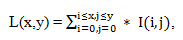
In order to perform any actions with data, the integral representation of images [3] is used in the Viola-Jones method. This representation is often used in other methods, for example, in wavelet transforms, SURF, and many other parsed algorithms. The integral representation allows you to quickly calculate the total brightness of an arbitrary rectangle in a given image, no matter what the rectangle is, the calculation time is constant.
The integral representation of the image is a matrix that is the same size as the original image . Each element of it contains the sum of the intensities of all pixels that are to the left and above the element . The elements of the matrix are calculated according to the following formula:
 (1.2)
(1.2)
where I (i, j) is the brightness of the pixel of the original image.
Each element of the matrix L [x, y] is the sum of pixels in the rectangle from (0,0) to (x, y), i.e. the value of each pixel (x, y) is equal to the sum of the values of all pixels to the left and above the given pixel (x, y). The matrix calculation takes linear time proportional to the number of pixels in the image, therefore the integral image is calculated in one pass.
The calculation of the matrix is possible according to the formula 1.3:
Using such an integral matrix, one can very quickly calculate the sum of the pixels of an arbitrary rectangle, of arbitrary area.
Suppose that in the rectangle ABCD there is an object D of interest to us:
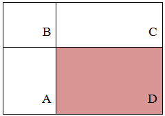
From the figure it is clear that the amount inside the rectangle can be expressed in terms of the sums and differences of adjacent rectangles by the following formula:
An approximate miscalculation is shown in the figure below:
The sign is the mapping f: X => D f , where D f is the set of valid values of the sign. If the attributes f 1 , ..., f n are given , then the feature vector x = (f 1 (x), ..., f n (x)) is called the feature description of the object x ∈ X. It is permissible to identify the feature descriptions with the objects themselves. Moreover, the set X = D f1 * ... * D fn is called the attribute space [1].
Signs are divided into the following types depending on the set D f :
Naturally, there are applied tasks with different types of signs, and not all methods are suitable for solving them.
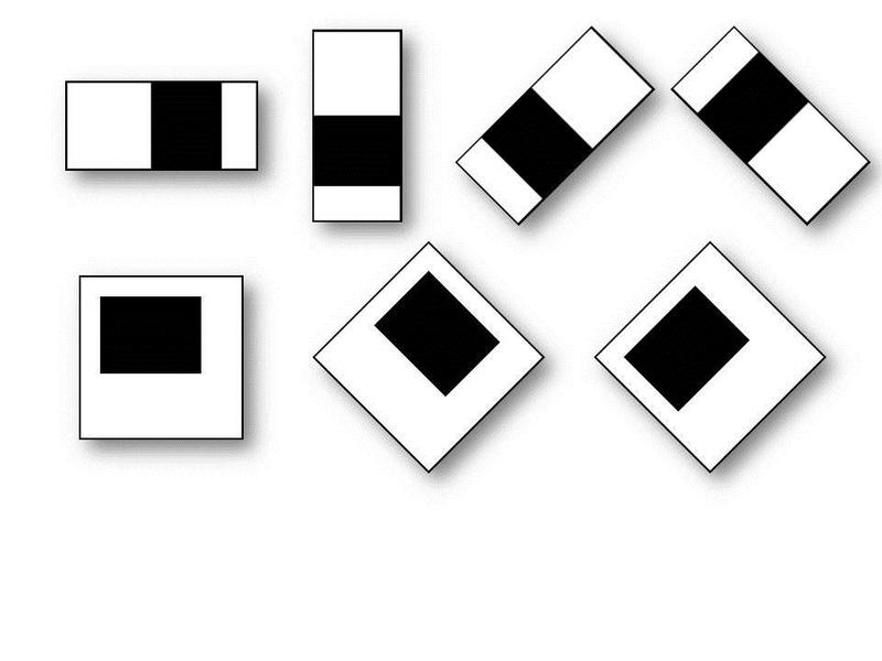
In the standard Viola-Jones method, the rectangular signs shown in the figure below are used, they are called Haar primitives :
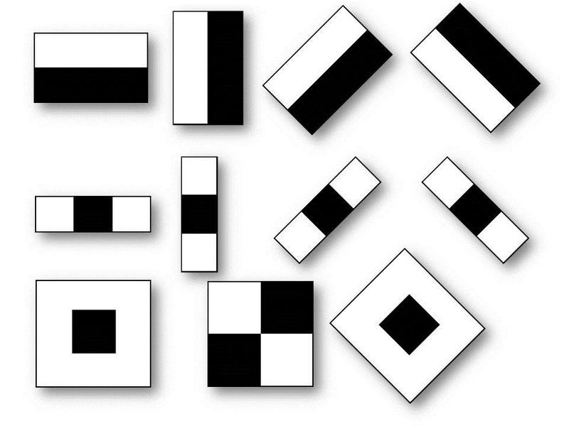
The advanced Viola-Jones method used in the OpenCV library uses additional features:
The calculated value of such a feature will be
where X is the sum of the brightness values of the points to be closed by the light part of the feature , and Y is the sum of the brightness values of the points to be closed by the dark part of the feature . To calculate them, the concept of an integral image, discussed above, is used.
The signs of Haar give a point value of the brightness difference along the X and Y axis, respectively .
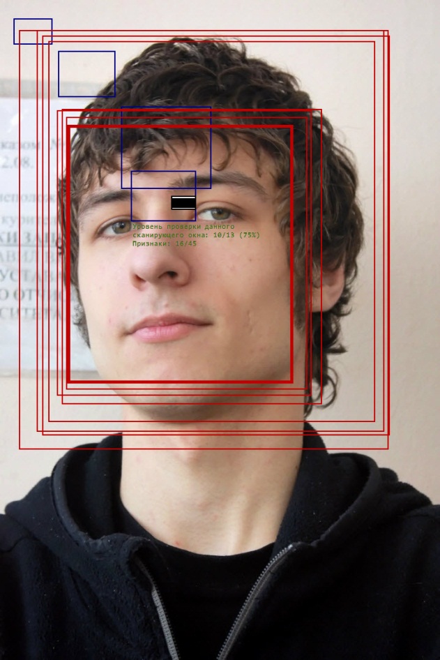
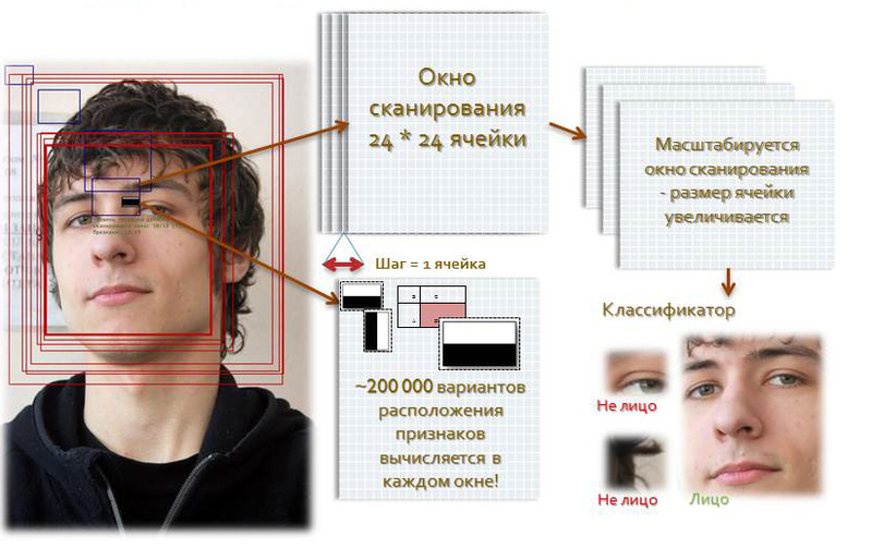
Visualization of the scanning window in the program:
The algorithm for scanning windows with signs looks like this:
In the search process to calculate all the signs on low-power desktop PCs is simply unrealistic. Consequently, the classifier should respond only to a specific, necessary subset of all features . It is quite logical that it is necessary to train the classifier in finding faces on this particular subset. This can be done by teaching the computer automatically .
Machine learning is the process by which a module gains new knowledge. There is a recognized definition for this process:
This process is part of the concept and technology called Data mining (information extraction and data mining) , which includes, besides Machine Learning, such disciplines as Database Theory, Artificial Intelligence, Algorithmization, Pattern Recognition, and others.
Machine learning in the Viola-Jones method solves such a problem as classification .
In the context of the algorithm, there are many objects (images), divided in some way into classes. A finite set of images is given for which it is known which class they belong to (for example, this could be the “frontal position of the nose” class). This set is called a training set. Class affiliation of other objects is not known. It is required to construct an algorithm capable of classifying an arbitrary object from the original set [4].
To classify an object means to indicate the number (or class name) to which the given object belongs.
Classification of an object - the number or name of the class, issued by the classification algorithm as a result of its application to this particular object.
Classifier - in classification problems, this is an approximating function that decides which particular class this object belongs to.
The training set is a finite amount of data.
In machine learning, the classification task is related to the training section with the teacher when the classes are divided . Pattern recognition is essentially a classification of images and signals. In the case of the Viola-Jones algorithm for face identification and recognition, the classification is two-class .
The classification is as follows:
There is X - a set in which the description of objects is stored, Y - a finite set of numbers belonging to classes. There is a dependency between them - the map Y *: X => Y. The training set is represented by
To solve the problem of this, so complex learning, there is a booster technology.
Boosting - a set of methods that contribute to improving the accuracy of analytical models. An effective model that admits few classification errors is called “strong . ” “Weak” , on the contrary, does not allow to reliably divide classes or give accurate predictions, it makes a lot of mistakes in the work. Therefore, boosting (from the English. Boosting - boosting, enhancing, improving) means literally “strengthening” the “weak” models [5] - this is a procedure for sequentially building the composition of machine learning algorithms, when each next algorithm seeks to compensate for the disadvantages of the composition of all previous algorithms.
The idea of boosting was proposed by Robert Shapir (Schapire) in the late 90s [6], when it was necessary to find a solution to the problem of having a lot of bad (slightly different from random) learning algorithms, to get one good one. The basis of this idea is the construction of a chain (ensemble) of classifiers [5, 6], which is called a cascade , each of which (except the first) learns from the mistakes of the previous one . For example, one of the first boosting algorithms Boost1 used a cascade of 3 models, the first of which was trained on the entire data set, the second on a sample of examples, in half of which the first gave correct answers, and the third on examples where “answers” the first two went their separate ways. Thus, there is a sequential processing of examples by a cascade of classifiers, and in such a way that the task for each subsequent one becomes more difficult. The result is determined by simple voting: the example refers to the class that is issued by most of the cascade models.
Busting is a greedy algorithm for constructing a composition of algorithms (greedy algorithm) - this is an algorithm that at every step makes the locally best choice in the hope that the final solution will be optimal. Boosting over decisive trees is considered one of the most effective methods in terms of classification quality. In many experiments, an almost unlimited decrease in the error rate was observed on an independent test sample as the composition was increased. Moreover, the quality of the test sample often continued to improve even after reaching the unmistakable recognition of the entire training sample. This turned the notion that existed for a long time that in order to increase the generalizing ability it is necessary to limit the complexity of the algorithms. Using the example of boosting, it became clear that arbitrarily complex compositions can have a good quality if properly tuned [5].
Mathematically, the boosting comes up like this:
Along with the sets X and Y, an auxiliary set R, called the estimate space , is introduced. We consider algorithms that have the form of a superposition a (x) = C (b (x)), where the function b: X → R is called an algorithmic operator , the function C: R → Y is the decision rule .
Many classification algorithms have exactly this structure: first, the estimates of the object's belonging to the classes are calculated, then the decision rule translates these estimates into the class number. The value of the assessment, as a rule, characterizes the degree of confidence of the classification.
Algorithmic composition - algorithm a: X → Y
composed of algorithmic operators b t : X → R, t = 1, ..., T, corrective operation F: R T → R and decision rule C: R → Y.
The basic algorithms denote the functions a t (x) = C (b t (x)), and for a fixed decision rule C, the operators b t (x) themselves.
Superpositions of the form F (b 1 , ..., b T ) are mappings from X to R, that is, again, algorithmic operators.
In classification problems into two non-intersecting classes, the set of real numbers is usually used as a rating space. Decision rules can have customizable parameters. So, in the Viola-Jones algorithm, the threshold decision rule is used , where, as a rule, an operator is first constructed at a zero value, and then the optimal value is chosen. The process of sequential learning of basic algorithms is probably used most often in the construction of compositions.
The stopping criteria can be used different, depending on the specifics of the task, it is also possible to apply several criteria together:
The development of this approach was the development of a more advanced AdaBoost family of algorithms for boosting ( adaptive boosting ), proposed by Yoav Freund (Freund) and Robert Schapire (1999), which can use an arbitrary number of classifiers and produce training on one set examples, alternately applying them to different steps.
The classification problem into two classes is considered, Y = {−1, + 1}. For example, the basic algorithms also return only two responses −1 and +1, and the decision rule is fixed: C (b) = sign (b). The desired algorithmic composition is:
 (1.7)
(1.7)
The quality functional of a composition Q t is defined as the number of errors it makes in the training set:
 (1.8)
(1.8)
where W l = (w 1 , ..., w l ) is the vector of object weights.
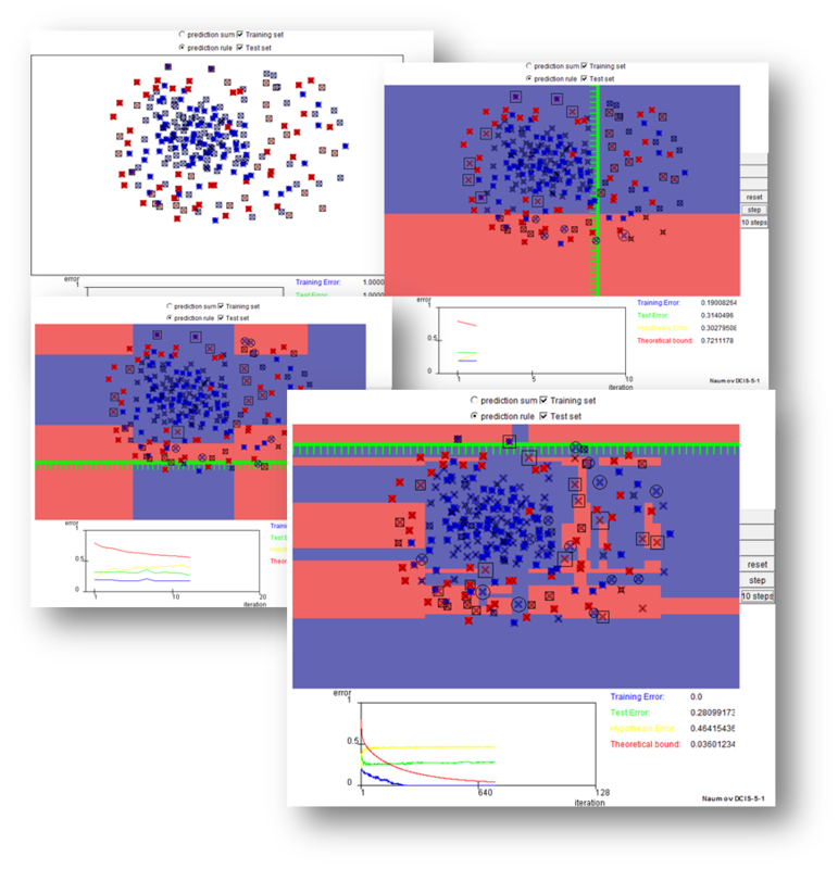
To solve the AdaBoosting problem, we need an exponential approximation of the threshold loss function [z <0], with the exponential E z = e -z (seen in the figure, which demonstrates the operation of AdaBoost below).
So, the general adaptive gain algorithm, AdaBoost, looks like this:
The implementation of AdaBoost at the preparatory stages of the 2nd step, the 12th and 642nd is shown in the figure. After constructing a certain number of basic algorithms (say, a couple dozen), it is necessary to analyze the distribution of object weights. The objects with the largest weights w i may be noise emissions, which should be excluded from the sample, and then start building the composition again.
AdaBoost advantages:
Cons AdaBoost:
Nowadays, the approach of strengthening simple classifiers is a popular and probably the most effective method of classification due to high speed and operational efficiency and relative ease of implementation.
A decision tree is a tree, in the leaves of which there are values of the objective function, and in the remaining nodes there are transition conditions (for example, there is a Smile on the Face), determining which of the edges to go. If, for a given observation, the condition is true, then a transition is made along the left edge, if false, then the right edge [4]. For example, the tree is shown in the following figure:

An example algorithm for creating a decision tree is shown below:
The advantages of such decisive trees are visibility, ease of working with them, speed. Also, they are easily applied to problems with many classes.
The algorithm for searching for faces from my point of view is this:
1. Definition of weak classifiers for rectangular features;
2. For each movement of the scanning window, a rectangular feature is calculated on each example;
3. Choose the most appropriate threshold for each feature;
4. The best signs and the best suitable threshold are selected;
5. Re-weighted sample.
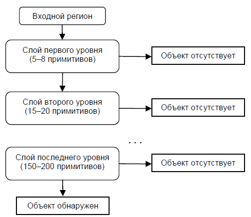
A cascading model of strong classifiers is essentially the same decision tree, where each tree node is designed to detect almost all images of interest and reject regions that are not images. In addition, the tree nodes are placed in such a way that the closer the node is to the root of the tree, the smaller number of primitives it consists of and thus requires less time to make a decision. This type of cascade model is well suited for image processing, in which the total number of detected images is small.
In this case, the method can quickly decide that the region does not contain an image, and proceed to the next one. An example of a cascade model of strong classifiers:
The complexity of learning such cascades is O (xyz), where x steps are used, y examples and z signs.
Further, the cascade is applied to the image:
1. Work with “simple” classifiers - in this case, part of the “negative” windows is discarded;
2. The positive value of the first classifier starts the second one, more adapted and so on;
3. The negative value of the classifier at any stage leads to an immediate transition to the next scanning window, the old window is discarded;
4. The chain of classifiers becomes more complex, so the errors become much smaller.
To train such a cascade will require the following steps:
1. Set the error level values for each stage (they must first be quantified when applied to the image from the training set) - they are called detection and false positive rates - it is necessary that the level of detection be high and the level of false positive rates low;
2. Signs are added until the parameters of the calculated stage reach the set level, here such auxiliary stages are possible as:
but. Testing additional small training set;
b.The AdaBoost threshold is deliberately lowered in order to find more objects, but in this regard, the greatest possible number of inaccurate definitions of objects;
3. If false positive rates remain high, then the next stage or layer is added;
4. False detections in the current stage are used as negative already in the next layer or stage.
In a more formal form, the cascade training algorithm is given below:
The mechanism of operation of the Viola-Jones algorithm was considered in detail. You can improve this method and modify it, which I achieved in my written program - this will be discussed in my next topic.
1. P. Viola and MJ Jones, “Rapid Object Detection using a Boosted Cascade of Simple Features”, IEEE Conf. on Computer Vision and Pattern Recognition (CVPR 2001), 2001
2. P. Viola and MJ Jones, “Robust real-time face detection,” International Journal of Computer Vision, vol. 57, no. 2, 2004., pp.137–154
3. R. Gonsales, R. Woods, “Digital Image Processing”, ISBN 5-94836-028-8, publishing house: Technosphere, Moscow, 2005. - 1072 p.
4. Mestetsky LM, “Mathematical methods of pattern recognition”, Moscow State University, Moscow, 2002–2004., P. 42 - 44
5. Jan ˇ Sochman, Jiˇr´ı Matas, AdaBoost, Center for Machine Perception, Czech Technical University, Prague, 2010
6. Yoav Freund, Robert E. Schapire, “A Short Introduction to Boosting”, Shannon Laboratory, USA, 1999., pp. 771-780
PS For the appearance of this article, I thank those people who pushed me the day before yesterday, and I got 2 karma points, and therefore the opportunity to present this article to HabraUzers. Have a great weekend everyone!
So, immediately to the point.
Viola Jones Method Description
The basic principles on which the method is based are:
- images are used in the integral representation , which allows you to calculate quickly the necessary objects;
- the signs of Haar are used , with the help of which the search for the necessary object takes place (in this context, the face and its features);
- use boosting (from the English. boost - enhancement, enhancement) to select the most appropriate signs for the desired object in this part of the image;
- all signs come to the input of the classifier , which gives the result “true” or “false”;
- feature cascades are used to quickly drop windows where no face has been found.
Training of classifiers is very slow, but face search results are very fast , which is why this method of face recognition in the image was chosen. Viola-Jones is one of the best in terms of performance indicators of recognition / speed. Also, this detector has an extremely low probability of false detection of the face. The algorithm even works well and recognizes facial features at a slight angle, up to about 30 degrees. When the angle of inclination is more than 30 degrees, the percentage of detections drops sharply. And it does not allow in the standard implementation to detect the rotated face of a person at an arbitrary angle, which greatly complicates or makes it impossible to use the algorithm in modern production systems, taking into account their growing needs.
A detailed analysis of the principles on which the Viola-Jones algorithm is based is required. This method generally looks for faces and facial features according to the general principle of a scanning window .
')
Scanning window principle
In general, the task of detecting a person’s face and facial features on a digital image looks like this:
- there is an image that has the desired objects . It is represented by a two-dimensional matrix of pixels of size w * h , in which each pixel has the value:
-0 255, if it is a black and white image;
-0 255 3, if it is a color image (components R, G, B). - as a result of its work, the algorithm should identify faces and their features and mark them - the search is performed in the active area of the image with rectangular signs , with the help of which the found face and its features are described:
rectangle i = {x,y,w,h,a},(1.1)
where x, y are the coordinates of the center of the i-th rectangle, w is the width, h is the height, a is the angle of inclination of the rectangle to the vertical axis of the image.
In other words, the scanning window (scanning window) approach is used for pictures and photographs: the image is scanned by the search window (the so-called scanning window), and then the classifier is applied to each position. The system of training and selection of the most significant features is fully automated and does not require human intervention, so this approach works quickly.
The task of finding and finding faces in an image with the help of this principle is often the next step on the way to recognizing characteristic features, for example, verifying a person by a recognized face or recognizing facial expressions.
Integral representation of images
In order to perform any actions with data, the integral representation of images [3] is used in the Viola-Jones method. This representation is often used in other methods, for example, in wavelet transforms, SURF, and many other parsed algorithms. The integral representation allows you to quickly calculate the total brightness of an arbitrary rectangle in a given image, no matter what the rectangle is, the calculation time is constant.
The integral representation of the image is a matrix that is the same size as the original image . Each element of it contains the sum of the intensities of all pixels that are to the left and above the element . The elements of the matrix are calculated according to the following formula:
(1.2)where I (i, j) is the brightness of the pixel of the original image.
Each element of the matrix L [x, y] is the sum of pixels in the rectangle from (0,0) to (x, y), i.e. the value of each pixel (x, y) is equal to the sum of the values of all pixels to the left and above the given pixel (x, y). The matrix calculation takes linear time proportional to the number of pixels in the image, therefore the integral image is calculated in one pass.
The calculation of the matrix is possible according to the formula 1.3:
L(x,y) = I(x,y) – L(x-1,y-1) + L(x,y-1) + L(x-1,y) (1.3)Using such an integral matrix, one can very quickly calculate the sum of the pixels of an arbitrary rectangle, of arbitrary area.
Suppose that in the rectangle ABCD there is an object D of interest to us:
From the figure it is clear that the amount inside the rectangle can be expressed in terms of the sums and differences of adjacent rectangles by the following formula:
S(ABCD) = L(A) + L() — L(B) — L(D) (1.4)An approximate miscalculation is shown in the figure below:
Signs of haar
The sign is the mapping f: X => D f , where D f is the set of valid values of the sign. If the attributes f 1 , ..., f n are given , then the feature vector x = (f 1 (x), ..., f n (x)) is called the feature description of the object x ∈ X. It is permissible to identify the feature descriptions with the objects themselves. Moreover, the set X = D f1 * ... * D fn is called the attribute space [1].
Signs are divided into the following types depending on the set D f :
- binary sign, D f = {0,1};
- nominal feature: D f - finite set;
- ordinal feature: D f - finite ordered set;
- quantitative attribute: D f - the set of real numbers.
Naturally, there are applied tasks with different types of signs, and not all methods are suitable for solving them.
In the standard Viola-Jones method, the rectangular signs shown in the figure below are used, they are called Haar primitives :
The advanced Viola-Jones method used in the OpenCV library uses additional features:
The calculated value of such a feature will be
F = XY , (1.5)where X is the sum of the brightness values of the points to be closed by the light part of the feature , and Y is the sum of the brightness values of the points to be closed by the dark part of the feature . To calculate them, the concept of an integral image, discussed above, is used.
The signs of Haar give a point value of the brightness difference along the X and Y axis, respectively .
Window scan
Visualization of the scanning window in the program:
The algorithm for scanning windows with signs looks like this:
- there is a test image, a scan window is selected, the used features are selected;
- then the scanning window starts to move sequentially through the image in 1 cell increments of the window (for example, the size of the window itself is 24 * 24 cells);
- when scanning an image in each window, approximately 200,000 variants of the location of signs are calculated by changing the scale of the signs and their position in the scanning window;
- scanning is performed sequentially for different scales;
- it is not the image itself that is scaled, but the scanning window (the cell size is changed);
- all found signs get to the classifier, which "makes a verdict."
In the search process to calculate all the signs on low-power desktop PCs is simply unrealistic. Consequently, the classifier should respond only to a specific, necessary subset of all features . It is quite logical that it is necessary to train the classifier in finding faces on this particular subset. This can be done by teaching the computer automatically .
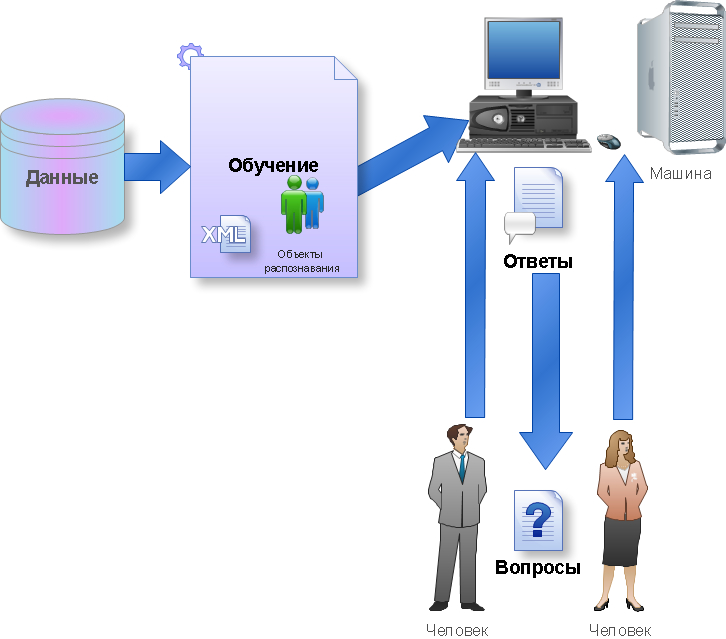
The machine learning model used in the algorithm
Machine learning is the process by which a module gains new knowledge. There is a recognized definition for this process:
“Machine learning is a science that studies computer algorithms that automatically improve during work” (Michel, 1996). Below is the learning process of the machine:
This process is part of the concept and technology called Data mining (information extraction and data mining) , which includes, besides Machine Learning, such disciplines as Database Theory, Artificial Intelligence, Algorithmization, Pattern Recognition, and others.
Machine learning in the Viola-Jones method solves such a problem as classification .
Classifier Training in Viola-Jones Method
In the context of the algorithm, there are many objects (images), divided in some way into classes. A finite set of images is given for which it is known which class they belong to (for example, this could be the “frontal position of the nose” class). This set is called a training set. Class affiliation of other objects is not known. It is required to construct an algorithm capable of classifying an arbitrary object from the original set [4].
To classify an object means to indicate the number (or class name) to which the given object belongs.
Classification of an object - the number or name of the class, issued by the classification algorithm as a result of its application to this particular object.
Classifier - in classification problems, this is an approximating function that decides which particular class this object belongs to.
The training set is a finite amount of data.
In machine learning, the classification task is related to the training section with the teacher when the classes are divided . Pattern recognition is essentially a classification of images and signals. In the case of the Viola-Jones algorithm for face identification and recognition, the classification is two-class .
The classification is as follows:
There is X - a set in which the description of objects is stored, Y - a finite set of numbers belonging to classes. There is a dependency between them - the map Y *: X => Y. The training set is represented by
X m = {(x 1 ,y 1 ), …, (x m ,y m )} . The function f is constructed from the feature vector X, which gives the answer for any possible observation X and is able to classify the object x∈X. This simple rule should work well on new data.AdaBoost used in the algorithm and development
To solve the problem of this, so complex learning, there is a booster technology.
Boosting - a set of methods that contribute to improving the accuracy of analytical models. An effective model that admits few classification errors is called “strong . ” “Weak” , on the contrary, does not allow to reliably divide classes or give accurate predictions, it makes a lot of mistakes in the work. Therefore, boosting (from the English. Boosting - boosting, enhancing, improving) means literally “strengthening” the “weak” models [5] - this is a procedure for sequentially building the composition of machine learning algorithms, when each next algorithm seeks to compensate for the disadvantages of the composition of all previous algorithms.
The idea of boosting was proposed by Robert Shapir (Schapire) in the late 90s [6], when it was necessary to find a solution to the problem of having a lot of bad (slightly different from random) learning algorithms, to get one good one. The basis of this idea is the construction of a chain (ensemble) of classifiers [5, 6], which is called a cascade , each of which (except the first) learns from the mistakes of the previous one . For example, one of the first boosting algorithms Boost1 used a cascade of 3 models, the first of which was trained on the entire data set, the second on a sample of examples, in half of which the first gave correct answers, and the third on examples where “answers” the first two went their separate ways. Thus, there is a sequential processing of examples by a cascade of classifiers, and in such a way that the task for each subsequent one becomes more difficult. The result is determined by simple voting: the example refers to the class that is issued by most of the cascade models.
Busting is a greedy algorithm for constructing a composition of algorithms (greedy algorithm) - this is an algorithm that at every step makes the locally best choice in the hope that the final solution will be optimal. Boosting over decisive trees is considered one of the most effective methods in terms of classification quality. In many experiments, an almost unlimited decrease in the error rate was observed on an independent test sample as the composition was increased. Moreover, the quality of the test sample often continued to improve even after reaching the unmistakable recognition of the entire training sample. This turned the notion that existed for a long time that in order to increase the generalizing ability it is necessary to limit the complexity of the algorithms. Using the example of boosting, it became clear that arbitrarily complex compositions can have a good quality if properly tuned [5].
Mathematically, the boosting comes up like this:
Along with the sets X and Y, an auxiliary set R, called the estimate space , is introduced. We consider algorithms that have the form of a superposition a (x) = C (b (x)), where the function b: X → R is called an algorithmic operator , the function C: R → Y is the decision rule .
Many classification algorithms have exactly this structure: first, the estimates of the object's belonging to the classes are calculated, then the decision rule translates these estimates into the class number. The value of the assessment, as a rule, characterizes the degree of confidence of the classification.
Algorithmic composition - algorithm a: X → Y
a(x) = C(F(b 1 (x), . . . , b T (x)), x ∈ X (1.6)composed of algorithmic operators b t : X → R, t = 1, ..., T, corrective operation F: R T → R and decision rule C: R → Y.
The basic algorithms denote the functions a t (x) = C (b t (x)), and for a fixed decision rule C, the operators b t (x) themselves.
Superpositions of the form F (b 1 , ..., b T ) are mappings from X to R, that is, again, algorithmic operators.
In classification problems into two non-intersecting classes, the set of real numbers is usually used as a rating space. Decision rules can have customizable parameters. So, in the Viola-Jones algorithm, the threshold decision rule is used , where, as a rule, an operator is first constructed at a zero value, and then the optimal value is chosen. The process of sequential learning of basic algorithms is probably used most often in the construction of compositions.
The stopping criteria can be used different, depending on the specifics of the task, it is also possible to apply several criteria together:
- built a specified number of basic algorithms T;
- Achieved accuracy on the training set;
- The achieved accuracy on the control sample has not been improved over the last few steps with a certain parameter of the algorithm.
The development of this approach was the development of a more advanced AdaBoost family of algorithms for boosting ( adaptive boosting ), proposed by Yoav Freund (Freund) and Robert Schapire (1999), which can use an arbitrary number of classifiers and produce training on one set examples, alternately applying them to different steps.
The classification problem into two classes is considered, Y = {−1, + 1}. For example, the basic algorithms also return only two responses −1 and +1, and the decision rule is fixed: C (b) = sign (b). The desired algorithmic composition is:
(1.7)The quality functional of a composition Q t is defined as the number of errors it makes in the training set:
(1.8)where W l = (w 1 , ..., w l ) is the vector of object weights.
To solve the AdaBoosting problem, we need an exponential approximation of the threshold loss function [z <0], with the exponential E z = e -z (seen in the figure, which demonstrates the operation of AdaBoost below).
So, the general adaptive gain algorithm, AdaBoost, looks like this:
:
Y = {−1,+1}, b 1 (x), . . . , b T (x) −1 + 1, X l – .
:
Y = {−1,+1}, b 1 (x), . . . , b T (x) −1 + 1, X l – .
:
Y = {−1,+1}, b 1 (x), . . . , b T (x) −1 + 1, X l – .:
Y = {−1,+1}, b 1 (x), . . . , b T (x) −1 + 1, X l – .
:
Y = {−1,+1}, b 1 (x), . . . , b T (x) −1 + 1, X l – .
:
1. :
w i := 1/ℓ, i = 1, . . . , ℓ; (1.9)
t = 1, . . . , T, :
2 .  (1.10)
2 .  (1.11)
3. . .  , b t , , b t x i . , , :
 (1.12)
4. :
 (1.13)
The implementation of AdaBoost at the preparatory stages of the 2nd step, the 12th and 642nd is shown in the figure. After constructing a certain number of basic algorithms (say, a couple dozen), it is necessary to analyze the distribution of object weights. The objects with the largest weights w i may be noise emissions, which should be excluded from the sample, and then start building the composition again.
AdaBoost advantages:
- good generalizing ability. In real problems, compositions are almost always constructed that exceed the basic algorithms in quality. Generalizing ability may improve as the number of basic algorithms increases;
- ease of implementation;
- own overhead expenses are small. The time to build a composition is almost completely determined by the learning time of the basic algorithms;
- the ability to identify objects that are noise emissions. These are the most "difficult" objects x i , for which in the process of increasing the composition, the weights w i take on the greatest values.
Cons AdaBoost:
- There is retraining in the presence of a significant level of noise in the data. The exponential loss function too much increases the weights of the “most difficult” objects, on which many basic algorithms are mistaken. However, it is these objects that most often turn out to be noise emissions. As a result, AdaBoost begins to tune in to noise, which leads to retraining. The problem is solved by removing outliers or using less “aggressive” loss functions. In particular, the GentleBoost algorithm is used;
- AdaBoost requires fairly long training samples. Other linear correction methods, in particular, bagging, are capable of building algorithms of comparable quality for smaller data samples;
- There is a construction of a non-optimal set of basic algorithms. To improve the composition, you can periodically return to the previously built algorithms and train them again.
- Boosting can lead to the construction of cumbersome compositions consisting of hundreds of algorithms. Such compositions exclude the possibility of meaningful interpretation, require large amounts of memory to store the basic algorithms and significant time spent on the calculation of classifications.
Nowadays, the approach of strengthening simple classifiers is a popular and probably the most effective method of classification due to high speed and operational efficiency and relative ease of implementation.
Principles of the decision tree in the developed algorithm
A decision tree is a tree, in the leaves of which there are values of the objective function, and in the remaining nodes there are transition conditions (for example, there is a Smile on the Face), determining which of the edges to go. If, for a given observation, the condition is true, then a transition is made along the left edge, if false, then the right edge [4]. For example, the tree is shown in the following figure:
An example algorithm for creating a decision tree is shown below:
function Node = _( {(x,y)} ) {
if {y}
return _(y);
test = __( {(x,y)} );
{(x0,y0)} = {(x,y) | test(x) = 0};
{(x1,y1)} = {(x,y) | test(x) = 1};
LeftChild = _( {(x0,y0)} );
RightChild = _( {(x1,y1)} );
return _(test, LeftChild, RightChild);
}
//
function main() {
{(X,Y)} = __();
TreeRoot = _( {(X,Y)} );
}
The advantages of such decisive trees are visibility, ease of working with them, speed. Also, they are easily applied to problems with many classes.
Cascade model of the developed algorithm
The algorithm for searching for faces from my point of view is this:
1. Definition of weak classifiers for rectangular features;
2. For each movement of the scanning window, a rectangular feature is calculated on each example;
3. Choose the most appropriate threshold for each feature;
4. The best signs and the best suitable threshold are selected;
5. Re-weighted sample.
A cascading model of strong classifiers is essentially the same decision tree, where each tree node is designed to detect almost all images of interest and reject regions that are not images. In addition, the tree nodes are placed in such a way that the closer the node is to the root of the tree, the smaller number of primitives it consists of and thus requires less time to make a decision. This type of cascade model is well suited for image processing, in which the total number of detected images is small.
In this case, the method can quickly decide that the region does not contain an image, and proceed to the next one. An example of a cascade model of strong classifiers:
The complexity of learning such cascades is O (xyz), where x steps are used, y examples and z signs.
Further, the cascade is applied to the image:
1. Work with “simple” classifiers - in this case, part of the “negative” windows is discarded;
2. The positive value of the first classifier starts the second one, more adapted and so on;
3. The negative value of the classifier at any stage leads to an immediate transition to the next scanning window, the old window is discarded;
4. The chain of classifiers becomes more complex, so the errors become much smaller.
To train such a cascade will require the following steps:
1. Set the error level values for each stage (they must first be quantified when applied to the image from the training set) - they are called detection and false positive rates - it is necessary that the level of detection be high and the level of false positive rates low;
2. Signs are added until the parameters of the calculated stage reach the set level, here such auxiliary stages are possible as:
but. Testing additional small training set;
b.The AdaBoost threshold is deliberately lowered in order to find more objects, but in this regard, the greatest possible number of inaccurate definitions of objects;
3. If false positive rates remain high, then the next stage or layer is added;
4. False detections in the current stage are used as negative already in the next layer or stage.
In a more formal form, the cascade training algorithm is given below:
a) f ( ) d ( )
b) F target
c) P –
d) N –
e) F 0 = 1,0; D 0 = 1,0; i = 0
f) while ( F i > F target )
i = i+1; n i = 0; F i = F i-1
while (F i = f * F i-1 )
n i = n i + 1
AdaBoost(P, N, n i )
F i D i ;
i- , d*D i -1 ( F i ) ;
g) N = Ø;
h) F i > F target , , , N.
findings
The mechanism of operation of the Viola-Jones algorithm was considered in detail. You can improve this method and modify it, which I achieved in my written program - this will be discussed in my next topic.
Bibliography:
1. P. Viola and MJ Jones, “Rapid Object Detection using a Boosted Cascade of Simple Features”, IEEE Conf. on Computer Vision and Pattern Recognition (CVPR 2001), 2001
2. P. Viola and MJ Jones, “Robust real-time face detection,” International Journal of Computer Vision, vol. 57, no. 2, 2004., pp.137–154
3. R. Gonsales, R. Woods, “Digital Image Processing”, ISBN 5-94836-028-8, publishing house: Technosphere, Moscow, 2005. - 1072 p.
4. Mestetsky LM, “Mathematical methods of pattern recognition”, Moscow State University, Moscow, 2002–2004., P. 42 - 44
5. Jan ˇ Sochman, Jiˇr´ı Matas, AdaBoost, Center for Machine Perception, Czech Technical University, Prague, 2010
6. Yoav Freund, Robert E. Schapire, “A Short Introduction to Boosting”, Shannon Laboratory, USA, 1999., pp. 771-780
PS For the appearance of this article, I thank those people who pushed me the day before yesterday, and I got 2 karma points, and therefore the opportunity to present this article to HabraUzers. Have a great weekend everyone!
Source: https://habr.com/ru/post/133826/
All Articles