Timsort sorting algorithm

Timsort , in contrast to all the “bubbles” and “inserts” there, is a relatively new thing - it was invented in 2002 by Tim Peters (named after him). Since then, it has already become the standard sorting algorithm in Python, OpenJDK 7 and Android JDK 1.5. And in order to understand why - just look at this tablet from Wikipedia.



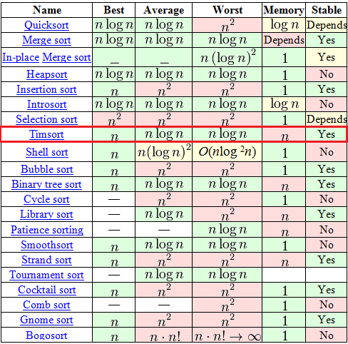
Among the seemingly huge choice in the table, there are only 7 adequate algorithms (with O (n logn) complexity on average and worst case), among which only 2 can boast of stability and O (n) complexity at best. One of these two is the well-known “Sorting with Binary Tree” for a long time. But the second one is Timsort.
')
The algorithm is built on the idea that in the real world a sorted data array often contains ordered (not important, ascending or descending) subarrays. This is indeed often the case. On such data Timsort tears to shreds all other algorithms.

Go to the point

Do not wait here for some complex mathematical discoveries. The fact is that in fact Timsort is not a completely independent algorithm, but a hybrid, an effective combination of several other algorithms, seasoned with its own ideas. Very briefly, the essence of the algorithm can be explained as follows:

1. By a special algorithm, we divide the input array into subarrays.
2. We sort each sub array in the usual sorting by inserts .
3. We assemble sorted subarrays into a single array using modified merge sorting .

The devil, as always, is hidden in the details, namely in the algorithm from item 1 and the modification of the merge sort from item 3.

Algorithm

Used concepts

• N is the size of the input array
• run - an ordered subarray in the input array. Moreover, it is ordered either weakly ascending or strictly descending. Ie or “a0 <= a1 <= a2 <= ...”, or “a0> a1> a2> ...”
• minrun - as mentioned above, in the first step of the algorithm, the input array will be divided into subarrays. minrun is the minimum size of such a subarray. This number is calculated according to a certain logic from the number N.

Step 0. Calculate minrun .

The minrun number is determined based on N based on the following principles:

1. It should not be too large, since sorting by inserts will be further applied to the minrun size array , and it is effective only on small arrays.
2. It should not be too small, because the smaller the subarray, the more iterations of subarray merging will have to be performed at the last step of the algorithm.
3. It would be nice if N \ minrun was a power of 2 (or close to it). This requirement is due to the fact that the subarray fusion algorithm works most effectively on subarrays of approximately equal size.

At this point, the author of the algorithm refers to his own experiments, which showed that if minrun > 256, point 1 is violated, when minrun <8, point 2 is broken and the values ​​from the range (32; 65) are used most effectively. The exception is if N <64, then minrun = N and timsort turns into simple sorting by insertion. At the moment, the minrun calculation algorithm is simply disgraceful: we take the upper 6 bits of N and add one if the remaining low bits have at least one non-zero one. Sample code looks like this:

int GetMinrun(int n) { int r = 0; /*  1        1  */ while (n >= 64) { r |= n & 1; n >>= 1; } return n + r; } 

Step 1. Splitting into subarrays and sorting them.

So, at this stage we have an input array, its size N and the calculated number minrun . The algorithm of this step:

1. We put the pointer of the current element at the beginning of the input array.
2. Starting with the current element, we look for the run in the input array (ordered subarray). By definition, this run will unambiguously enter the current element and the next one, but then further - as lucky as you are. If the resulting subarray is ordered in descending order, we rearrange the elements so that they go in ascending order (this is a simple linear algorithm, just go from both ends to the middle, changing the elements in places).
3. If the size of the current run 'is less than minrun - we take the elements in the number of minrun - size (run) that follow the run that it found. Thus, at the output we have a sub- array of minrun size or more, a part of which (and ideally it is all) is ordered.
4. Apply to this subarray sorting inserts. Since the size of the subarray is small and part of it is already ordered, the sorting works quickly and efficiently.
5. We set the current element pointer to the next element after the subarray.
6. If the end of the input array is not reached - go to step 2, otherwise - the end of this step.

Step 2. Merge.

At this stage, we have an input array, divided into subarrays, each of which is ordered. If the input array data were close to random - the size of the ordered subarrays is close to minrun , if the data were ordered ranges (and based on the recommendations on the application of the algorithm, we have reason to hope) - the ordered subarrays are larger than minrun .
Now we need to combine these subarrays to produce a resultant, fully ordered array. And in the course of this association, you need to fulfill 2 requirements:

1. Combine subarrays of approximately equal size (this is more efficient).
2. Preserve the stability of the algorithm - that is, do not make meaningless permutations (for example, do not change two consecutively the same number of places).

This is achieved in this way.

1. Create an empty stack of pairs <index of beginning of subarray> - <size of subarray>. Take the first ordered subarray.
2. We add to the stack a pair of data <start index> - <size> for the current subarray.
3. Determine if the current subarray should be merged with the previous ones. To do this, check the fulfillment of 2 rules (let X, Y and Z be the sizes of the three upper subarrays in the stack):
   X> Y + Z
   Y> Z
4. If one of the rules is violated, the array Y merges with the smaller of the arrays X and Z. Repeats until both rules are fulfilled or the data are completely ordered.
5. If there are still not considered subarrays, we take the next one and go to point 2. Otherwise, the end.

The purpose of this tricky procedure is to maintain balance. Those. The changes will look like this:

therefore, the sizes of the subarrays in the stack are effective for further merge sorting. Imagine the ideal case: we have subarrays of size 128, 64, 32, 16, 8, 4, 2, 2 (let's forget for a second about the presence of the requirement “size of subarray> = minrun ”). In this case, no merges will be executed until the last 2 subarrays meet, but after that 7 perfectly balanced mergers will be executed.

Subarray Merge Procedure

As you remember, in the second step of the algorithm we deal with the merging of two subarrays into one ordered one. We always connect 2 consecutive subarrays. Additional memory is used to merge them.

1. Create a temporary array in the size of the smallest of the connected subarrays.
2. Copy the smaller of the subarrays into a temporary array.
3. We put pointers to the current position on the first elements of a larger and temporary array.
4. At each next step, we consider the value of the current elements in the larger and temporary arrays, take the smaller of them and copy it into a new sorted array. Move the pointer of the current element in the array from which the element was taken.
5. Repeat 4 until one of the arrays is over.
6. Add all elements of the remaining array to the end of the new array.

Modification of the subarray fusion procedure

Everything seems to be good in the merge algorithm shown above. Except one. Imagine the procedure of merging two such arrays:
A = {1, 2, 3, ..., 9999, 10000}
B = {20000, 20001, ...., 29999, 30000}
The above procedure for them, of course, will work, but each time in its fourth paragraph you will need to perform one comparison and one copy. And that 10,000 comparisons and 10,000 copies. The Timsort algorithm offers a modification at this place, which he calls a "gallop." The bottom line is as follows:

1. Begin the merge procedure, as shown above.
2. On each operation of copying an element from a temporary or larger sub-array into the resulting one, we remember which sub-array was from which particular element.
3. If already a certain number of elements (in this implementation of the algorithm, this number is strictly equal to 7) was taken from the same array, we assume that we will have to take data from it further. To confirm this idea, we are switching to the “gallop” mode, i.e. We run through the array-applicant for the supply of the next large portion of data by binary search (we remember that the array is ordered and we have the full right to binary search) of the current element from the second array to be connected. Binary search is more efficient than linear, and therefore search operations will be much smaller.
4. Having finally found the moment when the data from the current supplier array no longer suits us (or by reaching the end of the array), we can finally copy them all at once (which can be more efficient than copying single elements).

Perhaps the explanation is slightly vague, try on an example.
A = {1, 2, 3, ..., 9999, 10000}
B = {20000, 20001, ...., 29999, 30000}

1. The first 7 iterations we compare the numbers 1, 2, 3, 4, 5, 6 and 7 from the array A with the number 20000 and, making sure that 20,000 is more - copy the elements of the array A into the resulting one.
2. Starting with the next iteration, we switch to the “gallop” mode: compare with the number 20000 successively the elements 8, 10, 14, 22, 38, n + 2 ^ i, ..., 10,000 of the array A. As you can see, such a comparison will be much less than 10,000.
3. We have reached the end of array A and know that it is all smaller than B (we could also stay somewhere in the middle). We copy the necessary data from array A into the resulting one, we go further.

That's the whole algorithm.

Materials on the topic

• Timsort on Wikipedia (no Russian version)
• Presentation of the algorithm from its creator
• Algorithm discussion on Stackoverflow
• Beautiful visualization algorithm