Hask category

Introduction

In this short article I will talk about category theory in the context of the Haskell type system. No zaumy, no tricks - I will try to explain everything clearly. I want to show the close connection of a programming language with mathematics in order to provoke the reader's awareness of one thing, through the other and vice versa.

I would not like to repeat the translation on this topic, which was already on Habré: Monads from the point of view of category theory , but for the integrity of the article, I will still give basic definitions. At the same time, unlike the article, I do not want to focus on mathematics.

This article largely repeats (including borrowing illustrations) a section from the English Haskell Wikibook , but nonetheless is not a direct translation.
')

What is a category?

Examples

For clarity, we first consider a couple of pictures depicting simple categories. They have red circles and arrows:

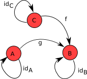
Red circles represent “objects”, and arrows - “morphisms”.

I want to give one illustrative example from real life, which will give some intuitive insight into the nature of objects and morphisms:

Cities can be considered “objects”, and movements between cities - “morphisms”. For example, you can imagine a flight map (I somehow did not find a good picture) or a railroad map - they will look like the pictures above, only more complicated. Attention should be paid to two points that seem to be taken for granted, but are important for the future:

• It happens that there is no way to get from one city to another by train or by plane - there are no morphisms between these cities.
• If we move within the same city, then this is also a morphism - we are traveling from the city to it, as it were.
• If there is a train from St. Petersburg to Moscow, and from Moscow there is a flight to Amsterdam, then we can buy a train ticket and a plane ticket, “combine” them and thus get from St. Petersburg to Amsterdam - that is, you can map draw an arrow from St. Petersburg to Amsterdam depicting this combined morphism.

I hope everything is clear with this example. And now a little formalism for clarity.

Definition

So, we already know that a category consists of objects and morphisms:

1. There is a class (set) of objects . Objects can be any entities.
2. For any two objects A and B , the class of morphisms Hom(A,B) defined. For a morphism f from this class, the object A is called a domain , and B is a co - domain . It is written like this:
   f ∈ Hom(A,B) or f : A → B
3. For any two morphisms f : A → B and g : B → C , their composition is defined — the morphism h = g ∘ f ,
   h : A → C It is important that the domain g and the domain f coincide.
4. The composition is associative , that is, for any morphisms f : A → B , g : B → C and h : C → D , the equality
   (h ∘ g) ∘ f = h ∘ (g ∘ f)
5. For any object A there is a “unit” morphism, which is denoted id A : A → A and it is neutral with respect to the composition, that is, for any morphism f : A → B satisfied:
   id B ∘ f = f = f ∘ id A

In the future, the index will bother me and I will write just id , since its area / area is restored from the context.

It can be verified that for the examples above, all the properties are fulfilled: the composition is defined when necessary, associative, and the corresponding isolated morphisms are neutral with respect to it. The only problem arises from the associativity in the example about moving between cities - here you need to think about the composition as “combining tickets”, and not just sequential movements of a particular person.

Exercise for self-test: check whether the following picture represents a category

Hask category

And now the main example, the main topic of the article. The Hask category consists of Haskell language types and functions between them. More strictly:

1. Hask objects: data types with ¹ * . For example, primitive types: Integer , Bool , Char , etc. The “Type” Maybe has a command * → * , but the type Maybe Bool has a command * and is therefore an object in Hask . The same with any parameterized types, but about them later. Notation: a ∷ * ≡ “type a has a keynd * ” ≡ “ a is an object in Hask ”.
2. Hask morphisms : any Haskell functions from one object (type) to another. If a, b ∷ * , then the function f ∷ a → b is a morphism with a domain a and a domain b . Thus, the class of morphisms between objects a and b is denoted by the type a → b . For completeness of the analogy with mathematical notation, we can introduce the following synonym:
   

    type Hom(a,b) = a → b 

   But I will not continue to use it, since the arrow, in my opinion, is clearer.
3. Composition: standard function (.) ∷ (b → c) → (a → b) → (a → c) . For any two functions f ∷ a → b and g ∷ b → c composition is g . f ∷ a → c g . f ∷ a → c is determined in a natural way:
   

    g . f = λx → g (fx) 

4. The composition associativity is obvious from this definition: For any three functions
   f ∷ a → b , g ∷ b → c and h ∷ c → d
   

    (h . g) . f ≡ h . (g . f) ≡ λx → h (g (fx)) 

   Direct check:

     (h . g) . f ≡ λx → (h . g) (fx) ≡ λx → (λy → h (gy)) (fx) ≡ λx → h (g (fx)) h . (g . f) ≡ λx → h ((g . f) x) ≡ λx → h ((λy → g (fy)) x) ≡ λx → h (g (fx)) 

5. For any type a ∷ * function id ∷ a → a is also defined in a natural way:
   

    id = λx → x 

   From this definition, the execution of the required properties is obvious. Let f ∷ a → b
   

    f . id ≡ λx → f (id x) ≡ λx → fx ≡ f id . f ≡ λx → id (fx) ≡ λx → fx ≡ f 

This function is polymorphic, so it is one for all, but from the point of view of a single morphism, we will perceive it as a separate morphism for each specific type, for example, for a Char object it will be a monomorphic function id ∷ Char → Char . That's why I said before about the index - in Haskell, you can not write every time what id we need, because its type is automatically taken out of context.

So, as we see, all the required entities are present, their interrelationships are presented, and the required properties are fulfilled, so Hask is a full-fledged category. Notice how all concepts and constructs are transferred from mathematical notation to Haskell with minimal syntactic changes.

Then I will talk about what functors are and how they are embodied in the category Hask .

Functors

Functors are transformations from one category to another. Since each category consists of objects and morphisms, the functor should consist of a pair of mappings: one will match objects from the first category to objects in the second, and the other will map to morphisms from the first category — morphisms to the second.

First I will give a mathematical definition, and then I will demonstrate how simple it becomes in the case of Haskell.

Mathematical definition

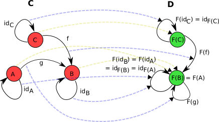
Consider two categories C and D and the functor F from C to D The notation used is the same as for morphisms, only the functor is denoted by a capital letter: F : C → D This F performs two roles:

1. Each object A from category C is associated with an object from category D and is denoted by F(A) .
2. Each morphism g : A → B from category C is associated with a morphism from category D and denoted by F(g) : F(A) → F(B) .

Once again, a functor is a pair of mappings:

  A ↦ F(A) g : A → B ↦ F(g) : F(A) → F(B) 

In the picture, the first display is depicted with yellow dotted arrows, and the second is blue:


The functor is required to fulfill two completely natural requirements:

1. He must translate every single morphism of a given object into a single morphism of its image:
   F(id A ) = id F(A)
2. He must translate the composition of morphisms into the composition of their images:
   F(h ∘ g) = F(h) ∘ F(g)

Functors in Hask

Now we look at functors from the Hask category in Hask . By the way, such functors that translate a category into it are called endofunctors .

So, then we need to translate types into types, and functions in functions are two mappings. And what is the construction language Haskell embodies the first? That's right, types with a knight * → * .

For example, the Maybe ∷ * → * type mentioned already Maybe ∷ * → * . This is a mapping that matches to any object a ∷ * an object from the same category (Maybe a) ∷ * . Here, Maybe a should be taken not as a constructor of a parameterized type with a given parameter a , but as a single character, similar to F(A) from a mathematical definition.

So, the first mapping comes to us for nothing - this is any type constructor with a parameter.

  data Maybe a = Nothing | Just a 

But how to get the second display? To do this, Haskell has a special class defined:

  class Functor f where fmap ∷ (a → b) → (fa → fb) 

where f ∷ * → * . That is, fmap is a polymorphic function that takes the morphism a → b , and returns the morphism fa → fb . Based on this, we will make Maybe real functor, defining the following function for it:

  instance Functor Maybe where fmap g = fg where fg Nothing = Nothing fg (Just x) = Just (gx) 

So, we got two maps:

  a ∷ * ↦ Maybe a ∷ * g ∷ a → b ↦ fmap g ∷ Maybe a → Maybe b 

There is nothing that, unlike mathematical notation, they have different names, it is just the specificity of the language, which does not affect the meaning.

Well, what about meeting the requirements? fmap must save the id and translate the composition into the composition:

  fmap id ≡ id fmap (h . g) ≡ (fmap h) . (fmap g) 

It is easy to verify this in the case of the above definition of fmap for Maybe .

Notice that we get the first mapping by simply declaring a type constructor with a parameter. And for him, as for the mapping between objects, it does not matter how the Maybe type is arranged: it simply associates with the object a object Maybe a , whatever that may be.

In the case of the display of morphisms, everything is not so simple: we have to manually define fmap , taking into account the Maybe structure. On the one hand, this gives us a certain flexibility - we decide how a function will transform a specific data structure. But on the other hand, it would be convenient to receive this definition for nothing, if we want it to be organized in a natural way. For example, for the type

  data Foo a = Bar a Int [a] | Buz Char Bool | Qux (Maybe a) 

the function g ∷ a → b should recursively bypass all data constructors and wherever they have a parameter of type a convert it with g . Moreover, if [a] or Maybe a is encountered, then their fmap g should work for them, which again bypasses their structure and transforms it.

And lo and behold, it is possible! GHC has a corresponding extension . We write in the code:

  {-# LANGUAGE DeriveFunctor #-} … data Foo a = … deriving Functor 

And we immediately get a full end - function of the category Hask - Foo , with the corresponding fmap .

By the way, it should be said that these functors actually map the Hask category into its subcategory , that is, into a category with a smaller class of objects and morphisms. For example, by displaying a ↦ Maybe a we can’t get a simple type Int - whatever a we took. Nevertheless, the resulting subclass of objects and the class of functions on them as morphisms also form a category.

In the Functor class documentation, you can also see a list of types for which the embodiment was originally defined. But they are mainly made in order to then say that this type is a monad.

Conclusion

So, I talked about the Hask category and the functors in it, and I hope it helped to realize the Haskell type system from a new perspective. Perhaps it seems useless from a practical point of view, since the meaning of fmap everyone probably understands in its own way and without knowing what a functor is. But then I’m going to write about natural transformations, monads and other categorical constructions in the key of the Hask category and then, I think, mathematical analogies will be more useful, allowing you to better understand the inner nature of these constructions of the language and apply them further more consciously.

---

1. If who did not meet earlier with kaynd (kinds), I will explain in two words. Kaynda is something like a type system over ordinary types. Kaynda are of two types:
   
   • * - this is a simple, not parameterized type. For example, Bool , Char , etc. Custom data Foo = Bar | Buz (Maybe Foo) | Quux [Int] type data Foo = Bar | Buz (Maybe Foo) | Quux [Int] data Foo = Bar | Buz (Maybe Foo) | Quux [Int] data Foo = Bar | Buz (Maybe Foo) | Quux [Int] will also be simple: Foo ∷ * , because the type constructor has no parameters (although its data constructors have)
   • … → … - this is a more complicated keynd, it can have any other keyes composed of * and → on the ground ellipsis. For example: [] ∷ * → * , or (,) ∷ * → (* → *) or anything else more complicated: ((* → *) → *) → (* → *) .
   
   The meaning of all this is simple: type constructors are kind of functions on types and describe how these functions interact correctly. For example, we cannot write [Maybe] , because [] ∷ * → * , that is, the argument of the parentheses must have a kand * , while Maybe it has * → * , that is, Maybe also a function and if we give it an argument Int ∷ * , then we get Maybe Int ∷ * and we can already pass it to the brackets: [Maybe Int] ∷ * . For this kind of control, the kayndas exist.