Analog computer on operational amplifiers
Analog computer is an analog computer (AVM), it is a continuous computer that processes analog data (continuous information).
TSB gives the definition of an analog computer.
An analogue computer (AVM), a computer in which each instantaneous value of a variable involved in the original ratios is assigned an instantaneous value of another (machine) quantity, often different from the original physical nature and scale factor. Each elementary mathematical operation on machine values, as a rule, corresponds to a certain physical law that establishes mathematical dependencies between the physical quantities at the output and input of the decision element (for example, Ohm and Kirchhoff's laws for electrical circuits, the expression for the Hall effect, Lorentz force, etc. .).
It should be noted that the analog computer is not only electric, but also mechanical, hydraulic and even pneumatic.
')
Despite the apparent anachronism, analog computing is widely used in modern life. Automotive automatic transmission is an example of a hydromechanical analogue transmitter, in which, when the torque changes, the fluid in the hydraulic actuator changes pressure, which makes it possible to obtain a change in transmission coefficient.
Analog processing of electrical signals occupies an important place in industrial electronics. Most types of primary transducers of physical quantities are sources of analog signals, and many actuators in control objects are controlled by a continuously varying electric current. Even control systems, which are based on digital computing systems, cannot abandon analog signal processing and interface with control objects and sensors using analog and analog-digital devices.
In connection with the bulk of the material that I would like to present, I plan to write a series of articles. I propose to the reader the first part, which will briefly tell the story of the creation of an operational amplifier as we know it.
The history of the use of AVM has several millennia. Those interested can start their search with an article in Wikipedia .
But in this article I will focus only on the dates, directly swinging the history of the creation of an electronic operational amplifier. And I will start with the date, which at first glance, does not relate to the topic of the article.
1614 Scottish mathematician John Napier publishes Canon on Logarithms, which began: “Realizing that there is nothing more boring and tedious in mathematics than multiplication, division, extraction of square and cubic roots, and that the operations mentioned are a waste of time and an inexhaustible source of elusive mistakes, I decided to find a simple and reliable means to get rid of them . "
Let me remind you about some properties of logarithms. From the properties of the logarithm, it follows that instead of time-consuming multiplication of many-valued numbers, it is enough to find (by tables) and add their logarithms, and then perform the potentiation on the same tables, that is, to find the result value by its logarithm. The execution of the division differs only in that the logarithms are subtracted.
In the form of formulas, it looks like this:
lg (xy) = lg (x) + lg (y) for multiplication
lg (x / y) = lg (x) - lg (y) to divide
Napier created the first logarithms of trigonometric functions.
Schoolchildren of the precomputer era must remember what four-digit Bradis tables are.
1622 English amateur mathematician William Redt created, perhaps, one of the most successful analog computing mechanism - a slide rule.
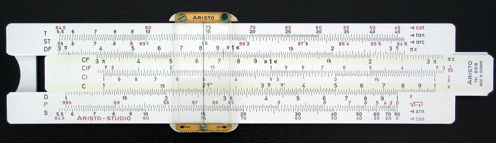
Fans of tinkering can collect their own pocket analog calculator with these instructions and learn how to use it until December 2012. Suddenly it will be useful ...
But still, I will skip the history of the development of non-electronic analog computers and go directly to the topic of our article.
1904 In November 1904, John Ambrose Fleming invented a rectifier on a two-electrode electron tube, which he called an oscillator valve. The invention also bears the name: a lamp with a thermal cathode, a vacuum diode, a kenotron, a thermionic lamp, a Fleming valve.
1906 The American Lee de Forest added a control “grid” to the electron tube and created a radio frequency detector called audion, but Fleming accused him of copying his ideas. De Forest's device was soon modified by him and Edwin Armstrong and used in the first electronic amplifier, and the lamp itself is called a triode .
1927 - Herold Steven Black at the Bell Telephone Laboratories research center creates an amplifier with negative feedback.

Fig. 1. Amplifier with negative feedback.
In essence, all electronic devices (electronic lamp, bipolar transistor, MOSFET) work nonlinearly. Negative feedback corrects this disadvantage by sacrificing gain for the sake of improving linearity (reducing distortion). But negative feedback can become positive under certain conditions, and then the amplifier will turn into a generator. Subsequently, Harry Nyquist developed a theory on how to make a stable OS.
30-40 years. In the 1930s, George A. Philbrick, working at the Foxboro Corporation, developed analog process control simulation models with vacuum tubes and passive elements. Philbrick developed many interesting circuits, and some were the ancestors of the operational amplifier.
Although amplifiers using both feedback and feedback were improved in the late 1930s and throughout the 1940s, several very interesting developments in the field of differential amplifiers are worth noting.
In the 30s there was a need for low level signals from living tissue. For this purpose, various tube amplifiers were used, such amplifiers were often called “biological amplifier”.
In 1934, V. HC Matthews , a biologist by profession, described a differential amplifier circuit. The amplifier did have differential inputs, but since the common cathodes were tied directly to the common power supply, it is not optimized to minimize the difference in the common-mode voltage at the inputs. Note that in those days common mode signals are often referred to as push-push signals, to designate phase signals at both inputs.
In 1936, Alan Blumlein developed the ideas of Matthews, by shifting the common cathodes of a differential pair through total resistance to the ground. Alan Blumlein received a patent for his amplifier, but the patent concerned broadband signals, not biological ones. However, this was a definite step forward compared to the Matthews amplifier, as it provides better detection of common-mode error. Diagrams of the Matthews and Blumlein amplifiers are shown in fig. 2

Fig. 2. Diagram of the differential amplifier.
1941 In the course of work on the gun data computer under the symbol M9 Bell Labs received a patent number 2,401,779 on the Summing amplifier .

Schematic diagram and component values for "Summing Amplifier"
US Patent 2,401,779, assigned to Bell Telephone Laboratories, Inc.)
Fig. 3. Scheme and list of components of the summing amplifier.
This design uses three vacuum tubes to achieve a gain of 90 dB and is controlled by a voltage of ± 350 V. The circuit has a single inverting input, rather than differential inverting and non-inverting inputs, as is often found in today's operational amplifiers. Using this scheme in the M9 military computer together with the SCR584 radar system yielded 90% accuracy of anti-aircraft fire. For the first time this system was used in 1944 during the landing of Allied forces in Italy .
1947 At the Columbia University in New York, the term operational amplifier (OU) was developed during research to improve analog computing for military purposes. Design OU was designed by Loebe Julie Loeb. This scheme had two major innovations. Funds have been applied to reduce the zero drift of the amplifier and, more importantly, it was the first design of the operational amplifier, which will have two inputs (one inverting, the other non-inverting).
1953. In 1946, after being discharged from the army, George A. Philbrick established a company named after himself, George A. Philbrick Researches, Inc., (GAP / R) and became involved in the creation of operational amplifiers. His work played an important role in the development of the OS.
Soon, in January 1953 , the first commercial OU K2-W was released. However, its cost was about $ 20. K2-W used two double 12AX7 triodes and was packaged in a standard eight-pin connector. OU was built on the design of Loeb Julie. Operating at a voltage of ± 300V, the op-amp could operate at output and input voltages up to ± 50V and had a gain of more than 15,000.
If the reader will have to create diagrams on this OS, then he can follow the links on page 1 , page 2 . For the rest, I'll just bring figure 4.


Fig.4. K2-W. Photography and electrical schematic diagram.
50 years. Tube amplifiers improved. Improved circuit solutions, increased gain, accuracy, reduced power consumption. But by the beginning of the 60s, the era of the warm tube opamp began to decline, and a transistor and, later, integrated circuits came on the scene.
1947 William Shockley , John Bardeen and Walter Brattein in Bell Labs laboratories for the first time created an active bipolar transistor , demonstrated on December 16th. On December 23, the official presentation of the invention took place and it is this date that is considered the day of invention of the transistor. By manufacturing technology, he belonged to the class of point transistors.
In May 1954. Gordon Thiel of Texas Instruments has developed a silicon transistor.
In 1958, Jack Kilby of Texas Instruments invented an integrated circuit, now known as a universal IC. Kilby's work, however, was not the only one. In early 1959, Robert Noyce , an engineer at Fairchild Semiconductor , also developed the concept of IP. After 10 years, in 1968, Robert Noyce and Gordon Moore will leave Fairchild Semiconductor and organize Intel , but this is another story.
The core of the concept of Noyce was actually closer to the concept of today's IP, as it uses the interconnection of metal layers between transistors and resistors. IP Kilby, by contrast, used the connection of the wires.
One of the versions of the history of creating IP is presented in an article in the Virtual Computer Museum .
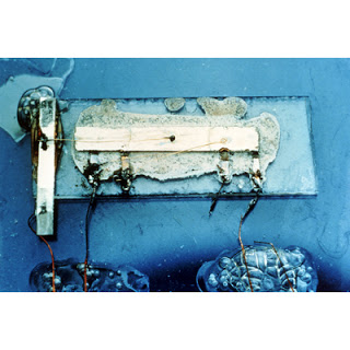
Fig. 5. Layout of the first Kilby IP.

Fig. 6. Illustration to the patent of Noyce.
1961 Anyway, as a result, in 1961, the first integrated circuits of operational amplifiers were produced. It was a GAP / R P45 worth about $ 120. These opamps were actually small circuit boards with edge connectors. As a rule, they were made up of carefully selected resistors in order to improve the characteristics of the OU, such as the bias voltage and the drift.
OU GAP / R P45 had a gain of 94 dB and was powered by a voltage of ± 15V. The op-amp had to deal with signals in the ± 10V range.
Later, these voltages became a kind of standard.


Fig. 7. OU GAP / R P45. Photography and electrical schematic diagram.
1961. George A. Philbrick creates a varactor bridge operational amplifier circuit.
In this circuit, the voltage of variable capacitors (varactors) is used in the input stage of the operational amplifier. As a result of the use of a varactor bridge, the lowest input current of any opamp was reached. Even less than the lamps.
Fig. 8 illustrates in the form of a block diagram varactor bridge OU. There are four main components, the front part consists of a bridge circuit and a high-frequency oscillator circuit, an AC amplifier for amplifying the bridge error voltage, a synchronous phase detector for converting the AC error current for the corresponding DC error, and finally, an output amplifier that provides additional DC amplification and load device.

Fig. 8. A block diagram of a varactor bridge operational amplifier.
The circuit works as follows: a small voltage error of the direct current Vin is applied to the selected varactor diodes D1 and D2 and causes an imbalance of the ac bridge, which is fed to the ac amplifier. This AC voltage will be phase shifted depending on the DC error voltage. The rest of the circuit amplifies and detects a DC error. Philbrick released the GAP / R P2 operational amplifier. Released in 1966, a modified op amp GAP / R SP2A could amplify an input current of the order of ± 10 pA (10 −12 ).
In 1965, Ray State Matthew Lorber created Analog Devices, Inc. (ADI) . Soon, Lewis R. Smith (Lewis R. Smith) created a varactor amplifier model 301, as well as its successors, models 310 and 311. These projects were able to achieve a significant increase in the accuracy of input currents to ± 10fA ( 10-15 ) below GAP / R P2). Interestingly, 310 and 311 models were sold at prices around $ 75. These amplifiers are still available in limited quantities.
1967 It is also worth noting that ADI has done a lot to popularize the use of OU. So, in 1967 she began to publish the magazine Analog Dialogue Magazine , which goes to this day. The online version of the magazine is a forum for the exchange of solutions in the field of circuit design and software for real devices and signal processing systems. It discusses technologies and methods for analog, digital and mixed signals. Working as an ADI technology gateway, Analog Dialogue is published monthly on the Internet. Selected technical articles are also presented in quarterly print publications .
1962 Alan Perlman and Roger Noble leave GAP / R and create a small company Nexus Research Laboratory, Inc. They were the first to launch OU packaged in rectangular modules with leads adapted for mounting on printed circuit boards. This design turned the Shelter into a “black box”, which was easily viewed as a separate element of the scheme. Modules have become so popular that GAP / R was forced to release its amplifier in a similar package.

Fig. 9. OU GAP / R PP65. Photography and electrical schematic diagram.
1963 μA702 of Fairchild Semiconductor Corporation was the first OU monolithic integrated circuit. μA702 was developed by a young engineer Robert J. (Bob) Vidlar . The professional activity of Vidlar over the course of just seven years (1963-1970) largely determined the development of analog microelectronics. But his μA702 definitely did not take the world by storm. It was not well received, because of unusual properties - excess supply voltage, low gain, etc. However, despite these shortcomings, some important design trends for IP were established for the μA702.
1965 μA709 released. It greatly improved the performance of the μA702. This is a higher gain (45,000 or ~ 94dB), expanded to ± 10V input / output voltage, reducing the input current to 200nA and increasing the output current. The amplifier was powered from a voltage of ± 15V. Frequency compensation was achieved by two RC chains between pins 1-8, and 6-5. The μA709 quickly became the standard and has been produced for several decades. Fig. 10 shows a schematic diagram of the μA709.
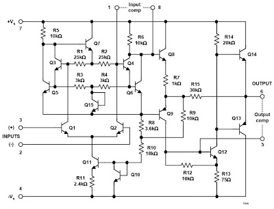
Fig. 10. Electrical circuit diagram μA709.
Despite the rather strong improvement in the circuit compared to the μA702, the amplifier still had problems.
1967. Not wanting to rest on the laurels of his OS μA702 and μA709, Bob Vidlar switched to another company, National Semiconductor Corporation (NSC). Its next integrated circuit design, the LM101 , was launched in 1967. The LM101 used a simple two-step topology that solved the μA709 problems. In addition, it was the design of operational amplifiers, which was subsequently followed by many manufacturers. A simplified diagram of the LM101 is shown in Figure 11.
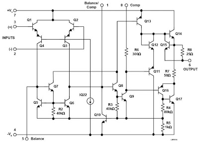
Fig. 11. Simplified diagram of the LM101.
The goals of the LM101 project were to eliminate such problems as μA709:
• No short circuit protection.
• Integrated frequency compensation.
• Sensitivity to overvoltage differential input.
• Excessive power dissipation and limited power range.
• Sensitivity to capacitive loads.
The new design of the LM101 solved the problems of the μA709, and added a few more improvements. Gain increased to 160,000 (~ 104 dB), useful power range increased from ± 5V to ± 20V. For easy upgrades, the LM101 used the same pins as the μA709 for input, output, and power.
1968 Less than a year after the release of the LM101, Fairchild in 1968 released the OA μA741 , designed by Dave Fallager. A simplified diagram of the μA741 is presented in Figure 12.
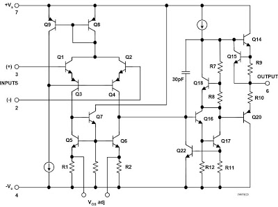
Fig. 12. Simplified scheme μA741.
Although there are obvious differences in the circuits, in μA741 the signal path is equivalent to LM101, and it provides similar behavior in terms of input short circuit and overvoltage protection, and has comparable bandwidth. A distinctive feature of the μA741 was the presence of a 30pF capacitor compensation in the chip, it soon became the standard.
The LM101, with the user-added capacitor, was functionally equivalent to the μA741. However, ease of use has proven to be more valuable to users than flexibility. National Semiconductor subsequently made a hybrid packet of an LM101 chip and a 30pF capacitor, but it was the μA741 that became the standard.
In Wikipedia this article is devoted to this amplifier.
1970 John AD Cadigan creates a high-speed operational amplifier. The distinctive ability of this opamp was the use of field-effect transistors in the input stage. OU was designed as a hybrid integrated circuit. Below, I will provide a diagram and a photograph of a more sophisticated op amp HQS-050 , released in 1977.

Fig. 13. HSQ-050. Electrical schematic diagram and photography.
I think that is worth staying at. And as a conclusion, I will cite another OU scheme that will allow us to evaluate the circuitry level of modern operational amplifiers.

Figure 14. AD549. Electrical schematic diagram.
In the second part, I will briefly review the internal circuitry of the operational amplifier.
The use of operational amplifiers as elements of analog computing devices will be presented in the third part.
The main source for this article was a book .
http://ru.wikipedia.org/wiki/
http://www.computer-museum.ru/
http://www.computerhistory.org/
TSB gives the definition of an analog computer.
An analogue computer (AVM), a computer in which each instantaneous value of a variable involved in the original ratios is assigned an instantaneous value of another (machine) quantity, often different from the original physical nature and scale factor. Each elementary mathematical operation on machine values, as a rule, corresponds to a certain physical law that establishes mathematical dependencies between the physical quantities at the output and input of the decision element (for example, Ohm and Kirchhoff's laws for electrical circuits, the expression for the Hall effect, Lorentz force, etc. .).
It should be noted that the analog computer is not only electric, but also mechanical, hydraulic and even pneumatic.
')
Despite the apparent anachronism, analog computing is widely used in modern life. Automotive automatic transmission is an example of a hydromechanical analogue transmitter, in which, when the torque changes, the fluid in the hydraulic actuator changes pressure, which makes it possible to obtain a change in transmission coefficient.
Analog processing of electrical signals occupies an important place in industrial electronics. Most types of primary transducers of physical quantities are sources of analog signals, and many actuators in control objects are controlled by a continuously varying electric current. Even control systems, which are based on digital computing systems, cannot abandon analog signal processing and interface with control objects and sensors using analog and analog-digital devices.
In connection with the bulk of the material that I would like to present, I plan to write a series of articles. I propose to the reader the first part, which will briefly tell the story of the creation of an operational amplifier as we know it.
Part one. Brief history of creating an operational amplifier.
The history of the use of AVM has several millennia. Those interested can start their search with an article in Wikipedia .
But in this article I will focus only on the dates, directly swinging the history of the creation of an electronic operational amplifier. And I will start with the date, which at first glance, does not relate to the topic of the article.
1614 Scottish mathematician John Napier publishes Canon on Logarithms, which began: “Realizing that there is nothing more boring and tedious in mathematics than multiplication, division, extraction of square and cubic roots, and that the operations mentioned are a waste of time and an inexhaustible source of elusive mistakes, I decided to find a simple and reliable means to get rid of them . "
Let me remind you about some properties of logarithms. From the properties of the logarithm, it follows that instead of time-consuming multiplication of many-valued numbers, it is enough to find (by tables) and add their logarithms, and then perform the potentiation on the same tables, that is, to find the result value by its logarithm. The execution of the division differs only in that the logarithms are subtracted.
In the form of formulas, it looks like this:
lg (xy) = lg (x) + lg (y) for multiplication
lg (x / y) = lg (x) - lg (y) to divide
Napier created the first logarithms of trigonometric functions.
Schoolchildren of the precomputer era must remember what four-digit Bradis tables are.
1622 English amateur mathematician William Redt created, perhaps, one of the most successful analog computing mechanism - a slide rule.
Fans of tinkering can collect their own pocket analog calculator with these instructions and learn how to use it until December 2012. Suddenly it will be useful ...
But still, I will skip the history of the development of non-electronic analog computers and go directly to the topic of our article.
1904 In November 1904, John Ambrose Fleming invented a rectifier on a two-electrode electron tube, which he called an oscillator valve. The invention also bears the name: a lamp with a thermal cathode, a vacuum diode, a kenotron, a thermionic lamp, a Fleming valve.
1906 The American Lee de Forest added a control “grid” to the electron tube and created a radio frequency detector called audion, but Fleming accused him of copying his ideas. De Forest's device was soon modified by him and Edwin Armstrong and used in the first electronic amplifier, and the lamp itself is called a triode .
1927 - Herold Steven Black at the Bell Telephone Laboratories research center creates an amplifier with negative feedback.
Fig. 1. Amplifier with negative feedback.
In essence, all electronic devices (electronic lamp, bipolar transistor, MOSFET) work nonlinearly. Negative feedback corrects this disadvantage by sacrificing gain for the sake of improving linearity (reducing distortion). But negative feedback can become positive under certain conditions, and then the amplifier will turn into a generator. Subsequently, Harry Nyquist developed a theory on how to make a stable OS.
30-40 years. In the 1930s, George A. Philbrick, working at the Foxboro Corporation, developed analog process control simulation models with vacuum tubes and passive elements. Philbrick developed many interesting circuits, and some were the ancestors of the operational amplifier.
Although amplifiers using both feedback and feedback were improved in the late 1930s and throughout the 1940s, several very interesting developments in the field of differential amplifiers are worth noting.
In the 30s there was a need for low level signals from living tissue. For this purpose, various tube amplifiers were used, such amplifiers were often called “biological amplifier”.
In 1934, V. HC Matthews , a biologist by profession, described a differential amplifier circuit. The amplifier did have differential inputs, but since the common cathodes were tied directly to the common power supply, it is not optimized to minimize the difference in the common-mode voltage at the inputs. Note that in those days common mode signals are often referred to as push-push signals, to designate phase signals at both inputs.
In 1936, Alan Blumlein developed the ideas of Matthews, by shifting the common cathodes of a differential pair through total resistance to the ground. Alan Blumlein received a patent for his amplifier, but the patent concerned broadband signals, not biological ones. However, this was a definite step forward compared to the Matthews amplifier, as it provides better detection of common-mode error. Diagrams of the Matthews and Blumlein amplifiers are shown in fig. 2
Fig. 2. Diagram of the differential amplifier.
1941 In the course of work on the gun data computer under the symbol M9 Bell Labs received a patent number 2,401,779 on the Summing amplifier .
Schematic diagram and component values for "Summing Amplifier"
US Patent 2,401,779, assigned to Bell Telephone Laboratories, Inc.)
Fig. 3. Scheme and list of components of the summing amplifier.
This design uses three vacuum tubes to achieve a gain of 90 dB and is controlled by a voltage of ± 350 V. The circuit has a single inverting input, rather than differential inverting and non-inverting inputs, as is often found in today's operational amplifiers. Using this scheme in the M9 military computer together with the SCR584 radar system yielded 90% accuracy of anti-aircraft fire. For the first time this system was used in 1944 during the landing of Allied forces in Italy .
1947 At the Columbia University in New York, the term operational amplifier (OU) was developed during research to improve analog computing for military purposes. Design OU was designed by Loebe Julie Loeb. This scheme had two major innovations. Funds have been applied to reduce the zero drift of the amplifier and, more importantly, it was the first design of the operational amplifier, which will have two inputs (one inverting, the other non-inverting).
1953. In 1946, after being discharged from the army, George A. Philbrick established a company named after himself, George A. Philbrick Researches, Inc., (GAP / R) and became involved in the creation of operational amplifiers. His work played an important role in the development of the OS.
Soon, in January 1953 , the first commercial OU K2-W was released. However, its cost was about $ 20. K2-W used two double 12AX7 triodes and was packaged in a standard eight-pin connector. OU was built on the design of Loeb Julie. Operating at a voltage of ± 300V, the op-amp could operate at output and input voltages up to ± 50V and had a gain of more than 15,000.
If the reader will have to create diagrams on this OS, then he can follow the links on page 1 , page 2 . For the rest, I'll just bring figure 4.
Fig.4. K2-W. Photography and electrical schematic diagram.
50 years. Tube amplifiers improved. Improved circuit solutions, increased gain, accuracy, reduced power consumption. But by the beginning of the 60s, the era of the warm tube opamp began to decline, and a transistor and, later, integrated circuits came on the scene.
1947 William Shockley , John Bardeen and Walter Brattein in Bell Labs laboratories for the first time created an active bipolar transistor , demonstrated on December 16th. On December 23, the official presentation of the invention took place and it is this date that is considered the day of invention of the transistor. By manufacturing technology, he belonged to the class of point transistors.
In May 1954. Gordon Thiel of Texas Instruments has developed a silicon transistor.
In 1958, Jack Kilby of Texas Instruments invented an integrated circuit, now known as a universal IC. Kilby's work, however, was not the only one. In early 1959, Robert Noyce , an engineer at Fairchild Semiconductor , also developed the concept of IP. After 10 years, in 1968, Robert Noyce and Gordon Moore will leave Fairchild Semiconductor and organize Intel , but this is another story.
The core of the concept of Noyce was actually closer to the concept of today's IP, as it uses the interconnection of metal layers between transistors and resistors. IP Kilby, by contrast, used the connection of the wires.
One of the versions of the history of creating IP is presented in an article in the Virtual Computer Museum .
Fig. 5. Layout of the first Kilby IP.
Fig. 6. Illustration to the patent of Noyce.
1961 Anyway, as a result, in 1961, the first integrated circuits of operational amplifiers were produced. It was a GAP / R P45 worth about $ 120. These opamps were actually small circuit boards with edge connectors. As a rule, they were made up of carefully selected resistors in order to improve the characteristics of the OU, such as the bias voltage and the drift.
OU GAP / R P45 had a gain of 94 dB and was powered by a voltage of ± 15V. The op-amp had to deal with signals in the ± 10V range.
Later, these voltages became a kind of standard.
Fig. 7. OU GAP / R P45. Photography and electrical schematic diagram.
1961. George A. Philbrick creates a varactor bridge operational amplifier circuit.
In this circuit, the voltage of variable capacitors (varactors) is used in the input stage of the operational amplifier. As a result of the use of a varactor bridge, the lowest input current of any opamp was reached. Even less than the lamps.
Fig. 8 illustrates in the form of a block diagram varactor bridge OU. There are four main components, the front part consists of a bridge circuit and a high-frequency oscillator circuit, an AC amplifier for amplifying the bridge error voltage, a synchronous phase detector for converting the AC error current for the corresponding DC error, and finally, an output amplifier that provides additional DC amplification and load device.
Fig. 8. A block diagram of a varactor bridge operational amplifier.
The circuit works as follows: a small voltage error of the direct current Vin is applied to the selected varactor diodes D1 and D2 and causes an imbalance of the ac bridge, which is fed to the ac amplifier. This AC voltage will be phase shifted depending on the DC error voltage. The rest of the circuit amplifies and detects a DC error. Philbrick released the GAP / R P2 operational amplifier. Released in 1966, a modified op amp GAP / R SP2A could amplify an input current of the order of ± 10 pA (10 −12 ).
In 1965, Ray State Matthew Lorber created Analog Devices, Inc. (ADI) . Soon, Lewis R. Smith (Lewis R. Smith) created a varactor amplifier model 301, as well as its successors, models 310 and 311. These projects were able to achieve a significant increase in the accuracy of input currents to ± 10fA ( 10-15 ) below GAP / R P2). Interestingly, 310 and 311 models were sold at prices around $ 75. These amplifiers are still available in limited quantities.
1967 It is also worth noting that ADI has done a lot to popularize the use of OU. So, in 1967 she began to publish the magazine Analog Dialogue Magazine , which goes to this day. The online version of the magazine is a forum for the exchange of solutions in the field of circuit design and software for real devices and signal processing systems. It discusses technologies and methods for analog, digital and mixed signals. Working as an ADI technology gateway, Analog Dialogue is published monthly on the Internet. Selected technical articles are also presented in quarterly print publications .
1962 Alan Perlman and Roger Noble leave GAP / R and create a small company Nexus Research Laboratory, Inc. They were the first to launch OU packaged in rectangular modules with leads adapted for mounting on printed circuit boards. This design turned the Shelter into a “black box”, which was easily viewed as a separate element of the scheme. Modules have become so popular that GAP / R was forced to release its amplifier in a similar package.
Fig. 9. OU GAP / R PP65. Photography and electrical schematic diagram.
1963 μA702 of Fairchild Semiconductor Corporation was the first OU monolithic integrated circuit. μA702 was developed by a young engineer Robert J. (Bob) Vidlar . The professional activity of Vidlar over the course of just seven years (1963-1970) largely determined the development of analog microelectronics. But his μA702 definitely did not take the world by storm. It was not well received, because of unusual properties - excess supply voltage, low gain, etc. However, despite these shortcomings, some important design trends for IP were established for the μA702.
1965 μA709 released. It greatly improved the performance of the μA702. This is a higher gain (45,000 or ~ 94dB), expanded to ± 10V input / output voltage, reducing the input current to 200nA and increasing the output current. The amplifier was powered from a voltage of ± 15V. Frequency compensation was achieved by two RC chains between pins 1-8, and 6-5. The μA709 quickly became the standard and has been produced for several decades. Fig. 10 shows a schematic diagram of the μA709.
Fig. 10. Electrical circuit diagram μA709.
Despite the rather strong improvement in the circuit compared to the μA702, the amplifier still had problems.
1967. Not wanting to rest on the laurels of his OS μA702 and μA709, Bob Vidlar switched to another company, National Semiconductor Corporation (NSC). Its next integrated circuit design, the LM101 , was launched in 1967. The LM101 used a simple two-step topology that solved the μA709 problems. In addition, it was the design of operational amplifiers, which was subsequently followed by many manufacturers. A simplified diagram of the LM101 is shown in Figure 11.
Fig. 11. Simplified diagram of the LM101.
The goals of the LM101 project were to eliminate such problems as μA709:
• No short circuit protection.
• Integrated frequency compensation.
• Sensitivity to overvoltage differential input.
• Excessive power dissipation and limited power range.
• Sensitivity to capacitive loads.
The new design of the LM101 solved the problems of the μA709, and added a few more improvements. Gain increased to 160,000 (~ 104 dB), useful power range increased from ± 5V to ± 20V. For easy upgrades, the LM101 used the same pins as the μA709 for input, output, and power.
1968 Less than a year after the release of the LM101, Fairchild in 1968 released the OA μA741 , designed by Dave Fallager. A simplified diagram of the μA741 is presented in Figure 12.
Fig. 12. Simplified scheme μA741.
Although there are obvious differences in the circuits, in μA741 the signal path is equivalent to LM101, and it provides similar behavior in terms of input short circuit and overvoltage protection, and has comparable bandwidth. A distinctive feature of the μA741 was the presence of a 30pF capacitor compensation in the chip, it soon became the standard.
The LM101, with the user-added capacitor, was functionally equivalent to the μA741. However, ease of use has proven to be more valuable to users than flexibility. National Semiconductor subsequently made a hybrid packet of an LM101 chip and a 30pF capacitor, but it was the μA741 that became the standard.
In Wikipedia this article is devoted to this amplifier.
1970 John AD Cadigan creates a high-speed operational amplifier. The distinctive ability of this opamp was the use of field-effect transistors in the input stage. OU was designed as a hybrid integrated circuit. Below, I will provide a diagram and a photograph of a more sophisticated op amp HQS-050 , released in 1977.
Fig. 13. HSQ-050. Electrical schematic diagram and photography.
I think that is worth staying at. And as a conclusion, I will cite another OU scheme that will allow us to evaluate the circuitry level of modern operational amplifiers.
Figure 14. AD549. Electrical schematic diagram.
In the second part, I will briefly review the internal circuitry of the operational amplifier.
The use of operational amplifiers as elements of analog computing devices will be presented in the third part.
List of used sources
The main source for this article was a book .
http://ru.wikipedia.org/wiki/
http://www.computer-museum.ru/
http://www.computerhistory.org/
Source: https://habr.com/ru/post/132702/
All Articles