Solution of the problem “Yandex Internet Mathematics - 2011”. Definition of visual similarity of images

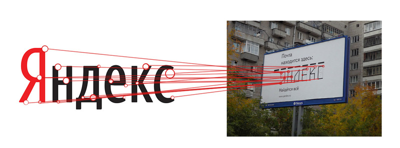In April-May 2011, Yandex conducted another round of the Yandex Internet Mathematics contest. Theme of the tour: "Determination of the visual similarity of images."
I published the news about the announcement of the winners and promised to soon describe the solution of the task set by our team - LookLikeIt, which took 12th place in the final ranking.

And now, not quite soon the time has come!

Introduction

Yandex Internet Mathematics is a series of contests organized by Yandex, which was held for the fifth time in 2011. The main content of the competition - competition in solving real problems based on real data. As a task for the competition in 2011, an analysis of the visual similarity of images was chosen to identify unnecessary frames in a series of panoramas. This article will describe the formulation of the problem, the methodology and approaches to its solution, which we used during the competition, as well as the analysis of the results obtained.
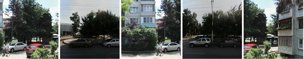
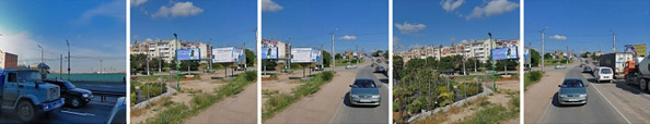
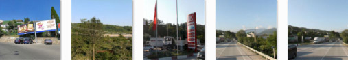
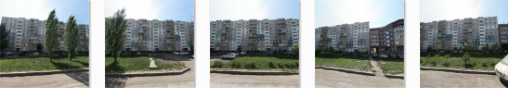
The data for the contest were images obtained from panoramic images of the Yandex.Maps service. The competition was divided into two stages - the training stage, which contained 6000 series of 5 images each (the dimension of each image was 300x300 pixels), and the final stage, which contained another set of 6000 series of 5 images each. The basis of each series is sequential fragments of a panorama with partial overlap (perhaps in the wrong order). Some series have one or two extra shots from other panoramic series. The task of the participants was using automatic methods to determine the extra frames in the series. Among the 6000 series of training set 1000 was a training sample, for which it was indicated which pictures are superfluous.
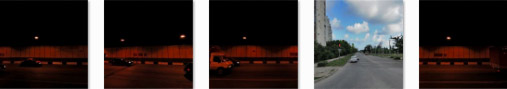
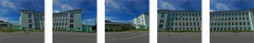
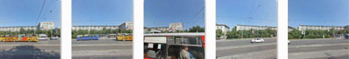
Examples of series:



The methodology of the competition was as follows. The teams made up the answer to the question: which photos are superfluous in each series of 5 photos for 5000 series at the training stage (from 1001 to 6000, since the first 1000 series were educational and the answers for it were known). This response was formed in the form of a text file, which indicated the extra images for each series. Based on this file, the Yandex server calculated a public assessment of the analysis results. At the final stage, a set of 6000 previously unknown series was proposed. The preliminary stage lasted 2 months, the final stage lasted exactly 24 hours (from May 16 to May 17, 2011).
The main metric for evaluating the results is the proportion of correctly classified photographs (two classes are considered: photographs constituting a panorama and superfluous). The evaluation was carried out according to the formula:
(Tp + Tn) / (P + N), where P is the number of images related to the panorama, N is the number of redundant images, Tp is the number of images that the system correctly related to the panorama, Tn is the number of images that the system correctly related to superfluous class. Thus, if the system absolutely correctly divided all photos into panorama and superfluous classes, then the estimate will be equal to 1.
After analyzing the metric it becomes clear that an error in the series can have a different effect on the overall assessment of the result. Consider the series presented in Figure 1. If the system says that 2,3,4,5 pictures are in the same panorama, and 1 is superfluous, then the estimate will be (3 + 1) / (3 + 2) = 4/5. If the system gives the result that 2, 3 and 4 pictures in one panorama, and 1 and 5 are superfluous, then the estimate will be (1 + 0) / (3 + 2) = 1/5. As can be seen from this, some types of errors can significantly degrade the overall assessment than others, which must be considered when designing a system.
The main tasks in developing a system to solve a problem were to determine metrics, based on which it is possible to determine whether two images are parts of the same panorama and the creation of a decision-making subsystem that, based on these metrics, will build the resulting answer for each series.
')

Metrics

In order to determine whether two images belong to the same panorama, we developed several types of metrics that are used in different situations. Images in one series are compared in pairs. Consider these metrics in more detail.

1. Overlay metric

In the formulation of the problem, the condition was specified that the images from one panorama should have a partial overlap. This is not always the case, but in most cases the overlap did take place.
To determine images with partial overlaps, we developed a method, the essence of which was as follows. The two images overlap each other with an overlay window width of 50 pixels.
In the resulting window, for each pixel, the difference is calculated modulo the RGB component, after which the relative number of pixels is calculated, for which the difference in R, G, and B values ​​is less than 20 for each component — we call such pixels “black”. This number indicates how close the colors were the pixels that were superimposed on each other and thus determines the degree of closeness of the superimposed portion of the first and second images.
After that, the window is shifted by 6 pixels and the procedure is repeated until the width of the overlay window increases to 150 pixels (half of the image). The same procedure is repeated for the same images with overlapping opposite sides (first, the right side of the first image on the left side of the second, and then - on the contrary, the right side of the second image on the left side of the first one).
For example, consider the image:

Let us show an iterative process of superimposing these images and calculating the difference of pixels in the overlay window:

Graph of changes in the relative number of dark pixels depending on the iteration of the overlay:

As you can see, at the 13th iteration we received a significant peak, and this means that we reached the overlap as precisely as possible, which is also confirmed by the illustration.
After this procedure for each pair of images in the series, we have two vectors with the values ​​of the relative number of “black” pixels and look for the maximum of them. This is the metric of proximity of two images by their partial overlap. In other words, we determine how strongly the two images coincide when they are superimposed on each other.
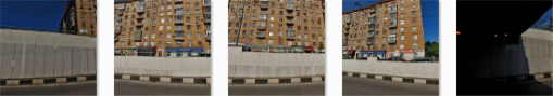
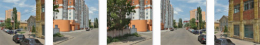
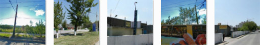
Obvious problems of this metric are initially dark images (night panoramas, etc.), since when a dark area is superimposed on a dark area, the difference in R, G, B values ​​will be small, despite the fact that there may not be a real overlap . To solve this problem, before starting the procedure, the total number of dark pixels in each image is checked, and if it is large enough (more than 70% of the image), then such a series is not analyzed using this metric. An example of such a series:

The second problem with the use of such a metric is images, the overlap of which is not exact, but has certain distortions:
-promising:

-the appearance of the object (machine) at the place of overlap:

-the presence of highly detailed objects at the site of overlap (trees, complex textures on buildings, glare), which cannot ideally “overlap” each other and give a high relative number of “black” pixels when applying the procedure described above:

In addition, despite the fact that the partial overlap was mentioned in the problem statement as a prerequisite for photos from the same panorama, a rather large number of series came across, where there was no overlap in the photos:

In this case, clarifying metrics were used, which will be described later.
The third problem associated with the overlay metric was determining the threshold of the metric (the maximum number of “black” pixels during the overlay passage on both sides), when it can be said that two images have a partial overlap or not.
The initial solution to this problem was the selection of a static threshold, the value of which was chosen by an empirical selection in a certain range of values ​​with a certain step along the training set. Thus, we obtained a certain value of the static threshold at which the result of a public assessment on the training sample was maximum. However, it is obvious that such an approach is not sufficiently effective, since the same threshold is not well suited for different series of photographs (for example, in series A for two photos, the overlap is pronounced and the metric gives a result of 95%, and in series B on the overlap of two There is a highly detailed object in the photos and the metric gives a result of 70%, which is quite small compared to 95% of Series A, but it can be much larger than other photos in Series B). In addition, the training set on which we picked up the threshold was rather small and not representative enough.
In connection with these problems, it was decided that the threshold for determining the proximity of the overlay metric must be calculated for each series separately. First, the metric value is calculated for all the photographs in the series in pairs, after which the mean square of these estimates is determined. The root mean square was chosen because of the fact that too high or too low values ​​are expressive and show a bright belonging of two photographs to the same panorama or vice versa, their difference is too great, therefore these peaks should have a greater effect on the average grade for the series using ascension square when calculating the average estimate. After that, each estimate is compared with the average estimate obtained, and if it is larger than it (with a certain margin), then the photos are considered to belong to the same panorama. If there is no such stock, it means that all the pictures in the series have approximately the same values, which may mean either that there are no extra pictures in this series, or that the metric did not work and it is necessary to specify the result further.
Using the approach of dynamic determination of the threshold for each series has improved the result of a public assessment of more than two-tenths.

2. Metrics of correlation of spectra

This metric was used for the series in which the overlap on the images from the same panorama was not obvious and was poorly determined using the overlay metric. In a fairly large number of series of images from the panorama and superfluous images were photographed under very different conditions (seasons, time of day, structure of the species (buildings and forests, for example), etc.), which gives a significant difference between them in the distribution of colors and brightness on images.

Therefore, to assess the similarity / difference in the distribution of colors, each picture from the series was decomposed into a spectrum (histogram) of 10 values: rainbow colors (red, orange, yellow, green, blue, blue, purple) and neutral colors: white, gray and black. For the colors of the rainbow, the HSV color space was used for the hue component (tone), which lies in the range of 0-360 values ​​and reflects the pixel tone. However, with this approach, without considering the brightness component in each under the color range, we will include white, gray and black colors, as shown in the figure:

Therefore, to exclude white, gray and black, first, the components of each pixel in the RGB space are checked for belonging to the ranges of these colors (for white, all components must be in the range: 225-255, for gray: 125-225, for black: 0- thirty).
Each component of the spectrum means the relative number of colors of one or another sub-range in the image, in other words, shows the distribution of colors in the image. It looks like this:

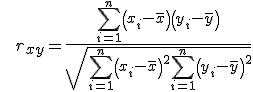
Since each spectrum is a vector of 10 values, to determine the existence of a relationship between the spectra of a pair of images in a series, the Pearson correlation coefficient was used:

This approach has proven itself very well, and the value of the correlation has grown rapidly for images, the color distribution of which was similar.

An important problem with this metric is, as with the overlay metric, the definition of a threshold that must cross the value of the correlation coefficient for two images to say that they belong to the same panorama. To solve this problem, a method was also used with a dynamic determination of the threshold for each series using the root-mean-square value of the correlation in the series.
The second problem is that there are series in which a photo from a panorama and an extra one have a very close distribution of colors (for example, the color of the sky and greenery), which gives false positives.

The third problem is images from a single panorama, on one of which a large object appears (for example, a passing car), which sometimes reaches half of the image. In this case, the spectral distribution for such an image varies greatly (a lot of blue appeared, for example, which was not on other images in the panorama) and the correlation cannot show the dependence of its spectrum with the spectra of other panorama images.

3. Metrics based on SURF descriptors

The SURF (Speeded Up Robust Features) method is one of the most efficient and fast modern algorithms for image recognition and determining their similarity.
The main point of the method is to select certain key points and small areas around them in the image. The key point is considered to be such a point, which has some signs that significantly distinguish it from the main mass of points. For example, it may be the edges of lines, small circles, sudden changes in illumination, angles, etc. Small areas around points are chosen because a small area of ​​the image is not very susceptible to perspective and large-scale distortion, but too small areas are also not suitable, since they contain too little information.
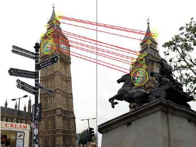
The SURF method searches for singular points using the Hesse matrix, whose determinant reaches an extremum at the points of maximum change in the brightness gradient and well detects spots, corners and edges of lines. Examples of key points:

This method is invariant to scale, rotations in the image plane, noise, overlapping other objects, changes in brightness and contrast. That is, ideal for those series that were problematic for the first two metrics.
The value of the metric when comparing two images was the number of common key points. We noted that when the number of points is more than ten - two images in the absolute majority of cases have common objects, because for this metric a static threshold was used, which practically did not give false positives.
This metric made it possible to determine those photos that were scaled in 360-degree panoramas, where the angles of view change too much and there are large perspective and geometric distortions, but the objects remain and remain key points. For example, in such series:


The main disadvantage of this method is a high computational load, and, consequently, a long time. However, we used it as a clarifier and calculated in the most problematic and controversial situations, so it was possible to reduce the number of calculations to a minimum.
As a method implementation, the OpenSURF 2.0 library was used.
You can read more about the SURF method in the wonderful article Detecting Sustainable Image Features: the SURF Method , from which we brazenly borrowed an illustration and description of the method :)

Decision making logic

Having developed metrics for pairwise comparison of images within a specific series and analyzing their advantages and disadvantages, as well as having conducted a series of tests on a training set, we created a decision-making subsystem which, based on these metrics, should form the answer: which photographs are superfluous in this series.
First, consider the possible variants of the series:
1) In a series of 3 photos in a panorama and 2 photos are superfluous;
a) extra photos in one panorama;
b) extra photos from different panoramas;
2) In a series of 4 photos in the panorama and 1 photo is superfluous;
3) No more;
Considering a series of photographs, the system creates two sets with pictures: mn.1 and mn.2. Initially, the algorithm distributes pictures to these sets, which among themselves exceed the dynamic threshold in the overlay metric. After that, the following logical variants of image distribution among these sets are possible. We describe the actions for these options:
1) (0) (0) - this option is not possible, since when using the dynamic threshold there are always images that have the imposition metric more than the average quadratic within this series (if the “stock” is not overcome in the imposition metric) sets using the spectra correlation metric, in which “margin” is not provided)
2) (2) (2) - this option means that the algorithm determined that two pictures are in the same panorama, two - in the other, but I could not say anything about the fifth one. In this case, the following options are possible:
A) the fifth will enter mn.1, and mn.2 will become redundant;
B) the fifth will enter mn.2, and mn.1 becomes redundant;
C) the fifth will go into both sets, then there will be no excess;
D) no metric can determine which set the fifth picture belongs to, because it analyzes the highest value of the correlation coefficient of this picture with pictures of the first set, second set, as well as the correlation coefficients of pictures from set 1 and set 2. Combining occurs according to the highest value of the coefficient spectral correlations:
- mn.1 and mn.2 unite and the 5th picture will be superfluous;
- pl.1 and 5th picture will unite and pl.2 will be superfluous;
- pl.2 and 5th picture will unite and pl.1 will be superfluous.
All adjustments are made on the metric of the spectrum correlation coefficient and the SURF method.

3) (3) (2) - it was empirically noted that in the training sample in the absolute majority of cases this option is right and clarification is not required (mn.2 - superfluous). In the case where this is not the case, the error will not be too gross and will not greatly affect the overall assessment of the result;
4) (2) (3) - similar to the previous paragraph (Pl. 1 - superfluous);
5) (3) (0) - in this case the following options are possible:
A) Both pictures are superfluous (option (3) (2));
B) one of the two pictures is included in the panorama, and the fifth one is superfluous (option (4) (1));
C) both pictures are included in the panorama, not superfluous (option (5) (0));
All adjustments are made on the metric of the spectrum correlation coefficient and the SURF method.

6) (4) (0) - in this case the options are possible:
A) The 5th picture is not included in the panorama, that is, the 5th is superfluous;
B) 5th picture is included in the panorama, there are no extras;
All adjustments are made on the metric of the spectrum correlation coefficient and the SURF method.

7) (5) (0) - no options. The answer is no extra.

Evaluation of results

The solution of the task set was carried out iteratively, using more and more complex approaches, gradually increasing the values ​​of the public assessment.
The greatest result was obtained by the solution described above and amounted to 0.945 on a preliminary public assessment. The final result increased to 0.967. The result of the winner in the final sample was 0.994.
The analysis of one series on average was about 20 seconds.
The main reason for such a sharp increase in the result in the final sample, in our opinion, is that the final set of the series was more thoroughly checked and there were practically no mistakes made by the compilers, which were often enough in the series of the preliminary stage.
Since this metric is not very clear and by its value the real recognition results are not very clear, we’ll give the statistics that we obtained in the training sample (such statistics can only be obtained on it, since the answers were known to it):
Absolutely correct answers: 85.3%; wrong answers with all sorts of errors: 14.7%.
This result is quite high. When analyzing the series that got into mistakes, we often came up against the fact that we ourselves could not determine the correct answer (or the correct, in our opinion, answer did not coincide with that of Yandex).
For example, in the series:

1 and 4 are redundant (although there is very little in common between images 2, 3 and 5).
And in this series:

only the first picture is considered superfluous. In our opinion, the fourth photo can be included in the same panorama with 2,3 and 5, and not go there and determine it is unrealistic.

After analyzing the results, we consider the insufficient number of metrics and the rigid logical structure of decision making to be the main drawbacks of the described solution. In fact, the training sample was used only to get a quick assessment of one method or another and collect statistics; no machine learning was provided for in the system. However, several leading teams, which at the preliminary stage occupied places in the first 5-ke, significantly reduced the result (from 0.975 to 0.941) in the final sample, due to the fact that their system was too much retrained in the preliminary data set.

I hope you were interested and you got to the end of this article :). Description of other solutions (including the decision of the winners) can be found here: Yandex Club .