Pseudorandom number generation
Quite often, programmers in their work are faced with the need to work with random numbers. Most often, random numbers are required in problems of modeling, numerical analysis and testing, but there are many other very specific tasks.
Of course, in all modern programming languages there is a function random or its analogs. These functions most often give really good pseudo-random numbers, but I always wondered how these functions work.
In this topic, I will try to explain how the linear congruent method works (which is most often used in the random function) and the method for obtaining random numbers using a polynomial counter (which is often used to test hardware).
It should immediately be said that it makes sense to generate random numbers only with a uniform distribution law, since all other distributions can be obtained from the uniform by transformations known from probability theory.
For those who have forgotten or have not yet studied probability theory, let me remind you that in a uniformly distributed sequence of zeroes and ones, zeroes on average (!) Will occur in 50% of cases. But this does not mean that in a sequence of 1000 digits there will be exactly 500 zeros. Moreover, in a sequence of 1000 digits there can be 999 zeros, and the probability that the thousandth element will be zero still remains equal to 0.5. At first glance, this seems paradoxical, but it is important to understand that all sequences are equally probable. If we consider a sufficiently large set of such sequences, then on average (!) In each of them there will be 500 zeros.
Having a little remembered the theory, we will pass to history. In precomputer times, random numbers were obtained by pulling colored balls out of bags, pulling cards, throwing dice. It is clear that serious studies could not be conducted this way, so in 1927 Tippett published the first table of random numbers. A little later, people tried to somehow automate this process. Random number machines began to appear. Now such devices are also used and are called entropy sources (generators). It is worth noting that only such devices can give truly random numbers. But, unfortunately, entropy generators are quite expensive, and it is not possible to install them in each PC. That is why there was a need for algorithms for obtaining random numbers.
Some people think that getting random numbers is easy. In their opinion, it is enough for this to do random complex mathematical operations on the original number. If we open the second volume of the well-known Knut, we will learn that in 1959 Knut also tried to build a generator based on such an idea. His algorithm looked like this:
K1. [Select the number of iterations.] Assign Y to the largest significant digit of X. (We will perform steps K2-K13 exactly Y + 1 times, i.e., apply randomized transformations a random number of times.)
K2. [Select a random step] Assign the next most significant digit X. Go to step K (3 + Z), i.e., to a randomly selected step in the program.
KZ [Provide> 5 x 10⁹] If X <5000000000, assign X the value X + 5000000000.
K4. [The middle of the square.] Replace X with the middle of the square X.
K5. [Multiply.] Replace X with the number (1001001001 X) mod 1010.
K6. [Pseudo-completion.] If X <100000000, then assign X the value X + 9814055677; otherwise, assign X to the value 1010- X.
K7. [Rearrange the halves.] Swap the five lower-order characters with the older ones.
K8. [Multiply.] Perform step K5.
K9. [Shrink digits.] Shrink each non-zero decimal number of X by one.
K10. [Modify to 99999.] If A '<105, assign the X value to X 2 +99999; otherwise, assign X to X - 99999.
K11. [Normalize.] (At this step, A 'cannot be zero.) If X <109, then multiply X by 10.
K12. [Modification of the center square method.] Replace X with the average 10 digits of the number X (X - 1).
K13 [Repeat?] If Y> 0, decrease Y by 1 and return to step K2. If Y = 0, the algorithm is complete. The value of the number X obtained in the previous step will be the desired "random" value.
Despite the apparent complexity, this algorithm quickly came down to the number 6065038420, which in a small number of steps was transformed into itself. The moral of this story is that you cannot use a random algorithm to get random numbers.
In most programming languages, this method is used in the standard function for obtaining random numbers. This method was first proposed by Lehmer in 1949. Choose 4 numbers:
The sequence is obtained using the following recurrent formula: X n + 1 = (a * X n + c) mod m.
This method gives really good pseudo-random numbers, but if we take the numbers m, a, c arbitrarily, the result will most likely disappoint us. When m = 7, X 0 = 1, a = 2, c = 4, we get the following sequence: 1,6,2,1,6,2,1, ...
Obviously, this sequence does not quite fit the definition of random. However, this failure allowed us to draw two important conclusions:
In fact, any function that maps a finite set of X to X will produce cyclically repeated values. So our task is to maximize the unique part of the sequence (by the way, it is obvious that the length of the unique part cannot be greater than m).
Without going into details of the evidence, let's say that the period of the sequence will be equal to m only if the following three conditions are met:
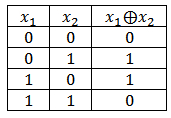
The algorithm that we are going to consider is based on the operation of the exclusive OR (the sum modulo two). Just in case, let me remind you what the truth table looks like for this function:
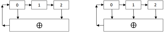
The schemes shown in the figure below are the simplest polynomial counters. The zero bit in such schemes is calculated based on the exclusive OR function, and all other bits are obtained by a simple shift. Discharges from which the signal goes to the exclusive OR are called bends.
Consider how the values in these registers will change with the initial value 001:
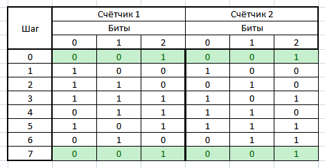
Both registers start working from the same value, but then the values generated by the registers begin to diverge quickly. But after 6 steps, both registers are returned to their original state.
It is easy to show that both of these registers generated the longest possible sequence that contains all the combinations except the zero one. Those. when the register is m, you can get a sequence of length 2 m -1.
A polynomial counter of any digit capacity has a number of combinations of taps, which will ensure a sequence of maximum length, the use of incorrect combinations will lead to the generation of short sequences. A separate and rather difficult task is to search for these combinations of taps.
It is worth noting that these combinations are not always unique. For example, for a 10-bit counter there are two of them: [6; 9] and [2; 9]; for a six-digit counter there are twenty-eight such combinations.
In order to find these combinations, it is necessary to present the counter as a polynomial. The counters from the example will look like this: x 2 XOR 1 and x 2 XOR x XOR 1.
')
It is known from theory that a necessary and sufficient condition for the generation of a complete sequence is the primitiveness of the characteristic polynomial. It means that:
The advantages of a polynomial counter are simplicity, both software and hardware implementation, speed and cryptographic strength.
Hope this article was helpful to you.
Of course, in all modern programming languages there is a function random or its analogs. These functions most often give really good pseudo-random numbers, but I always wondered how these functions work.
In this topic, I will try to explain how the linear congruent method works (which is most often used in the random function) and the method for obtaining random numbers using a polynomial counter (which is often used to test hardware).
Introduction
It should immediately be said that it makes sense to generate random numbers only with a uniform distribution law, since all other distributions can be obtained from the uniform by transformations known from probability theory.
For those who have forgotten or have not yet studied probability theory, let me remind you that in a uniformly distributed sequence of zeroes and ones, zeroes on average (!) Will occur in 50% of cases. But this does not mean that in a sequence of 1000 digits there will be exactly 500 zeros. Moreover, in a sequence of 1000 digits there can be 999 zeros, and the probability that the thousandth element will be zero still remains equal to 0.5. At first glance, this seems paradoxical, but it is important to understand that all sequences are equally probable. If we consider a sufficiently large set of such sequences, then on average (!) In each of them there will be 500 zeros.
Having a little remembered the theory, we will pass to history. In precomputer times, random numbers were obtained by pulling colored balls out of bags, pulling cards, throwing dice. It is clear that serious studies could not be conducted this way, so in 1927 Tippett published the first table of random numbers. A little later, people tried to somehow automate this process. Random number machines began to appear. Now such devices are also used and are called entropy sources (generators). It is worth noting that only such devices can give truly random numbers. But, unfortunately, entropy generators are quite expensive, and it is not possible to install them in each PC. That is why there was a need for algorithms for obtaining random numbers.
First attempt to obtain a memory bandwidth
Some people think that getting random numbers is easy. In their opinion, it is enough for this to do random complex mathematical operations on the original number. If we open the second volume of the well-known Knut, we will learn that in 1959 Knut also tried to build a generator based on such an idea. His algorithm looked like this:
K1. [Select the number of iterations.] Assign Y to the largest significant digit of X. (We will perform steps K2-K13 exactly Y + 1 times, i.e., apply randomized transformations a random number of times.)
K2. [Select a random step] Assign the next most significant digit X. Go to step K (3 + Z), i.e., to a randomly selected step in the program.
KZ [Provide> 5 x 10⁹] If X <5000000000, assign X the value X + 5000000000.
K4. [The middle of the square.] Replace X with the middle of the square X.
K5. [Multiply.] Replace X with the number (1001001001 X) mod 1010.
K6. [Pseudo-completion.] If X <100000000, then assign X the value X + 9814055677; otherwise, assign X to the value 1010- X.
K7. [Rearrange the halves.] Swap the five lower-order characters with the older ones.
K8. [Multiply.] Perform step K5.
K9. [Shrink digits.] Shrink each non-zero decimal number of X by one.
K10. [Modify to 99999.] If A '<105, assign the X value to X 2 +99999; otherwise, assign X to X - 99999.
K11. [Normalize.] (At this step, A 'cannot be zero.) If X <109, then multiply X by 10.
K12. [Modification of the center square method.] Replace X with the average 10 digits of the number X (X - 1).
K13 [Repeat?] If Y> 0, decrease Y by 1 and return to step K2. If Y = 0, the algorithm is complete. The value of the number X obtained in the previous step will be the desired "random" value.
Despite the apparent complexity, this algorithm quickly came down to the number 6065038420, which in a small number of steps was transformed into itself. The moral of this story is that you cannot use a random algorithm to get random numbers.
Linear congruential method
In most programming languages, this method is used in the standard function for obtaining random numbers. This method was first proposed by Lehmer in 1949. Choose 4 numbers:
- Module m (m> 0);
- The factor a (0 <= a <m);
- Increment c (0 <= c <m);
- The initial value of X 0 (0 <= X 0 <m)
The sequence is obtained using the following recurrent formula: X n + 1 = (a * X n + c) mod m.
This method gives really good pseudo-random numbers, but if we take the numbers m, a, c arbitrarily, the result will most likely disappoint us. When m = 7, X 0 = 1, a = 2, c = 4, we get the following sequence: 1,6,2,1,6,2,1, ...
Obviously, this sequence does not quite fit the definition of random. However, this failure allowed us to draw two important conclusions:
- The numbers m, a, c, X 0 should not be random;
- The linear congruential method gives us repeated sequences.
In fact, any function that maps a finite set of X to X will produce cyclically repeated values. So our task is to maximize the unique part of the sequence (by the way, it is obvious that the length of the unique part cannot be greater than m).
Without going into details of the evidence, let's say that the period of the sequence will be equal to m only if the following three conditions are met:
- The numbers c and m are coprime;
- a-1 is a multiple of p for each simple p that is a divisor of m;
- If m is a multiple of 4, then a-1 must be a multiple of 4.
Getting pseudo-random numbers based on a polynomial counter (shift register)
The algorithm that we are going to consider is based on the operation of the exclusive OR (the sum modulo two). Just in case, let me remind you what the truth table looks like for this function:
The schemes shown in the figure below are the simplest polynomial counters. The zero bit in such schemes is calculated based on the exclusive OR function, and all other bits are obtained by a simple shift. Discharges from which the signal goes to the exclusive OR are called bends.
Consider how the values in these registers will change with the initial value 001:
Both registers start working from the same value, but then the values generated by the registers begin to diverge quickly. But after 6 steps, both registers are returned to their original state.
It is easy to show that both of these registers generated the longest possible sequence that contains all the combinations except the zero one. Those. when the register is m, you can get a sequence of length 2 m -1.
A polynomial counter of any digit capacity has a number of combinations of taps, which will ensure a sequence of maximum length, the use of incorrect combinations will lead to the generation of short sequences. A separate and rather difficult task is to search for these combinations of taps.
It is worth noting that these combinations are not always unique. For example, for a 10-bit counter there are two of them: [6; 9] and [2; 9]; for a six-digit counter there are twenty-eight such combinations.
In order to find these combinations, it is necessary to present the counter as a polynomial. The counters from the example will look like this: x 2 XOR 1 and x 2 XOR x XOR 1.
')
It is known from theory that a necessary and sufficient condition for the generation of a complete sequence is the primitiveness of the characteristic polynomial. It means that:
- The characteristic polynomial cannot be represented as a product of polynomials of a lower degree;
- The characteristic polynomial is a divisor of the polynomial z δ XOR 1, with (δ = 2 m -1, and is not a divider with any other values δ <2 m -1.
The advantages of a polynomial counter are simplicity, both software and hardware implementation, speed and cryptographic strength.
Hope this article was helpful to you.
Source: https://habr.com/ru/post/132217/
All Articles