RMS approximation of functions

The other day it was necessary to write a program that calculates the root-mean-square approximation of a function given in tabular form, according to a power basis - by the least squares method. At once I will make a reservation that I did not consider the trigonometric basis and I will not take it in this article. At the end of the article you can find the source code of the program in C #.

Theory

Let the values ​​of the approximated function f (x) be given at N + 1 nodes f (x ₀ ), ..., f (x _N ) . The approximating function will be chosen from some parametric family F (x, c) , where c = (c ₀ , ..., c _n ) ^T is the parameter vector, N> n .

The principal difference in the task of the mean square approximation from the interpolation problem is that the number of nodes exceeds the number of parameters. In this case, there is almost always no such vector of parameters for which the values ​​of the approximating function would coincide with the values ​​of the approximated function in all nodes.

In this case, the problem of approximation is posed as the problem of finding such a vector of parameters c = (c ₀ , ..., c _n ) ^T , at which the values ​​of the approximating function deviate as little as possible from the values ​​of the approximated function F (x, c) in the aggregate of all knots.
')
Graphically, the task can be represented as


We write the rms approximation criterion for the least squares method:
J (c) = √ (Σ _{i = 0} ^N [f (x _i ) - F (x, c)] ² ) → min

The root expression is a quadratic function with respect to the coefficients of the approximating polynomial. It is continuous and differentiable with respect to c ₀ , ..., c _n . Obviously, its minimum is at the point where all partial derivatives are zero. Equating the partial derivatives to zero, we obtain a system of linear algebraic equations for the unknown (desired) coefficients of the best approximation polynomial.

The least squares method can be applied to various parametric functions, but often in engineering practice polynomials are used as an approximating function for some linearly independent basis { φ _k (x), k = 0, ..., n }:
F (x, c) = Σ _{k = 0} ⁿ [ c _k φ _k (x) ] .

In this case, the system of linear algebraic equations for determining the coefficients will have a completely specific form:
a ₀₀ c ₀ + a ₀₁ c ₁ +… + a _0n c _n = b ₀
a ₁₀ c ₀ + a ₁₁ c ₁ +… + a _1n c _n = b ₁
...
a _n0 c ₀ + a _n1 c ₁ +… + a _nn c _n = b _n

a _kj = Σ _{i = 0} ^N [φ _k (x _i ) φ _j (x _i )], b _j = Σ _{i = 0} ^N [f (x _i ) φ _j (x _i )]

For this system to have a unique solution, it is necessary and sufficient that the determinant of the matrix A (the Gram determinant) be non-zero. In order for the system to have a unique solution, it is necessary and sufficient that the system of basic functions φ _k (x), k = 0, ..., n be linearly independent on the set of approximation nodes.

In this article, we consider the root-mean-square approximation by polynomials in the power basis { φ _k (x) = x ^k , k = 0, ..., n }.

Example

And now for the example. It is required to derive an empirical formula for the given tabular dependence f (x) using the least squares method.

x	0.75	1.50	2.25	3.00	3.75
y	2.50	1.20	1.12	2.25	4.28

Take as an approximating function
y = F (x) = c ₀ + c ₁ x + c ₂ x ² , i.e., n = 2, N = 4

The system of equations for determining the coefficients:
a ₀₀ c ₀ + a ₀₁ c ₁ +… + a _0n c _n = b ₀
a ₁₀ c ₀ + a ₁₁ c ₁ +… + a _1n c _n = b ₁
...
a _n0 c ₀ + a _n1 c ₁ +… + a _nn c _n = b _n

a _kj = Σ _{i = 0} ^N [φ _k (x _i ) φ _j (x _i )], b _j = Σ _{i = 0} ^N [f (x _i ) φ _j (x _i )]

The coefficients are calculated by the formulas:
a ₀₀ = N + 1 = 5, a ₀₁ = Σ _{i = 0} ^N x _i = 11.25, a ₀₂ = Σ _{i = 0} ^N x _i ² = 30.94
a ₁₀ = Σ _{i = 0} ^N x _i = 11.25, a ₁₁ = Σ _{i = 0} ^N x _i ² = 30.94, a ₁₂ = Σ _{i = 0} ^N x _i ³ = 94.92
a ₂₀ = Σ _{i = 0} ^N x _i ² = 30.94, a ₂₁ = Σ _{i = 0} ^N x _i ³ = 94.92, a ₂₂ = Σ _{i = 0} ^N x _i ⁴ = 303.76
b ₀ = Σ _{i = 0} ^N y _i = 11.25, b ₁ = Σ _{i = 0} ^N x _i y _i = 29, b ₂ = Σ _{i = 0} ^N x _i ² y _i = 90.21

We solve the system of equations and obtain the following coefficients:
c ₀ = 4.822, c ₁ = -3.882, c ₂ = 0.999

In this way
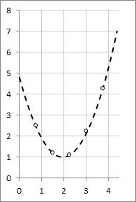
y = 4.8 - 3.9x + x ²

Graph of the resulting function

C # release

And now let's move on to how to write code that would build such a matrix. And here, it turns out, everything is quite simple:

private double[,] MakeSystem(double[,] xyTable, int basis) { double[,] matrix = new double[basis, basis + 1]; for (int i = 0; i < basis; i++) { for (int j = 0; j < basis; j++) { matrix[i, j] = 0; } } for (int i = 0; i < basis; i++) { for (int j = 0; j < basis; j++) { double sumA = 0, sumB = 0; for (int k = 0; k < xyTable.Length / 2; k++) { sumA += Math.Pow(xyTable[0, k], i) * Math.Pow(xyTable[0, k], j); sumB += xyTable[1, k] * Math.Pow(xyTable[0, k], i); } matrix[i, j] = sumA; matrix[i, basis] = sumB; } } return matrix; } 

At the input, the function receives a table of function values ​​— a matrix, the first column of which contains the values ​​of x, the second, respectively, y, as well as the value of the power basis.

First, the memory is allocated for the matrix, in which the coefficients for solving a system of linear equations will be written. Then, in fact, we compose a matrix — in sumA, the values ​​of the coefficients aij are written, in sumB - bi, all according to the formula specified above in the theoretical part.

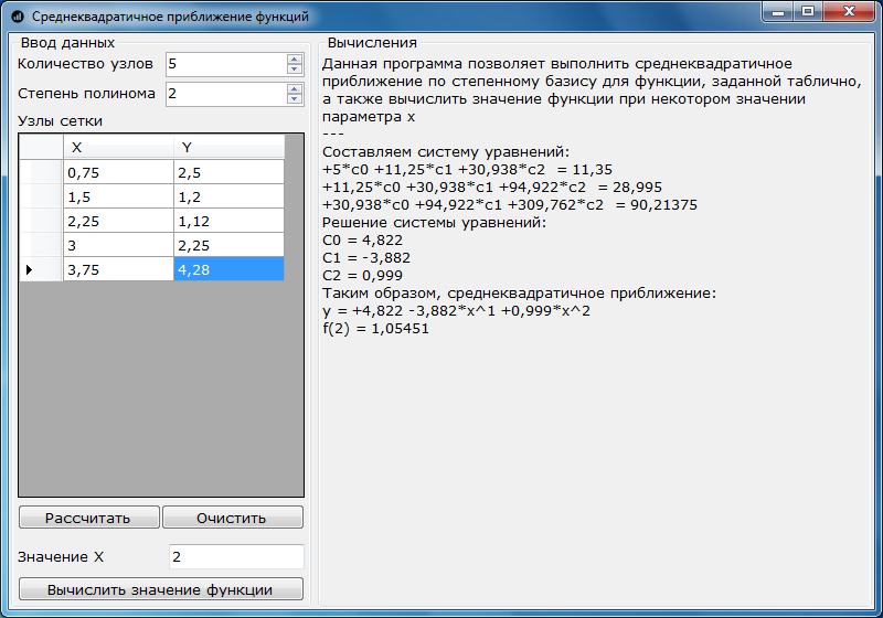
To solve the compiled system of linear algebraic equations in my program, the Gauss method is used. The archive with the project can be downloaded here .

Screenshot of the program on the example solved above:



Sources used:
Sulimova V.V. Guidelines for the course "Computational Workshop" - Tula, TSU, 2009 - 65 p.