The abbreviation OFDM stands for Orthogonal frequency-division multiplexing. In the Russian-language literature there are several different translations that carry, in principle, one sense: OFDM is a multiplexing (compaction) mechanism by means of orthogonal subcarriers.

The article describes the pros and cons of the mechanism of OFDM. The principle of functioning from a physical and mathematical position is considered. The article contains an introductory description of the radiophysical terms necessary for understanding the material to a wide range of readers.

Illustration: 18, characters: 27 399, lines of code: 99.

In the specifications of the latest telecommunications wired and wireless standards, it is increasingly possible to find the use of OFDM technology. Requirements to architectures of radio systems dictate by time provide high popularity. The OFDM mechanism has a number of properties that allow to meet the trends of the time. Developed back in the 60s of the last century, the technology became available for use only relatively recently.

OFDM materials are sufficient in Russian. On Habré, for example, you can read a good article from the company Yota . A list of some sources is given at the end of the article.

The presentation of the material is designed for readers with different levels of training. Therefore, in order to speak a common language, the introductory material is presented in the first half of the article. An experienced reader can go directly to the second half of the article, where it will be discussed directly about OFDM. For those who are only interested in the answer to the question raised in the title, you can read only a couple of first paragraphs below.

Why does WiMax and LTE use OFDM?

The secret lies in the features of the technology, you can briefly highlight the main positive and negative sides:

• High efficiency of using the radio frequency spectrum, explained by the almost rectangular shape of the spectrum envelope with a large number of subcarriers.
• Simple hardware implementation: basic operations are implemented using digital processing methods.
• Good resistance to intersymbol interference (ISI - intersymbol interference) and interference between subcarriers (ICI - intercarrier interference). As a result - loyalty to multipath propagation.
• The possibility of using different modulation schemes for each subcarrier, which allows adaptively varying noise immunity and information transfer rate.

• High frequency and time synchronization is required.
• Sensitivity to the Doppler effect, limiting the use of OFDM in mobile systems.
• Not ideal modern receivers and transmitters causes phase noise, which limits the performance of the system.
• The guard interval used in OFDM to combat multipath propagation reduces the spectral efficiency of the signal.

Despite all the shortcomings, OFDM is an excellent solution for architectures of modern networks operating in the metropolis. Technical progress and market dynamics are constantly pushing manufacturers to improve existing technologies. As a result, devices appear that rely on various OFDM modifications. However, the core and the principles laid down in it remain the same. The surface fundamentals of the functioning of OFDM technology are discussed in this article.

Step 1. About spectra

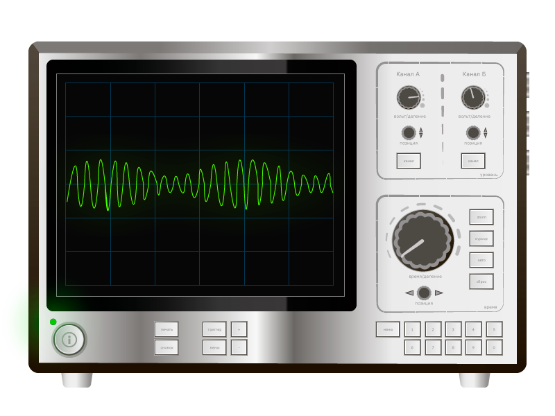
Consider the signal shown in the figure below.

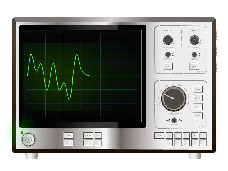
For convenience, only one period (one repetition cycle) of the signal is given. A signal is a change in voltage over time at some point in an electrical circuit. The creation, transmission and reception of such changes are the essence of radio electronics.

Looking at the change in voltage over time, a number of conclusions can be made. If it is, for example, a signal from a sensor, then the graph describes the dynamics of the measured value. However, modern radio engineering mostly speaks the language of spectra. To help realize this concept can figure below.

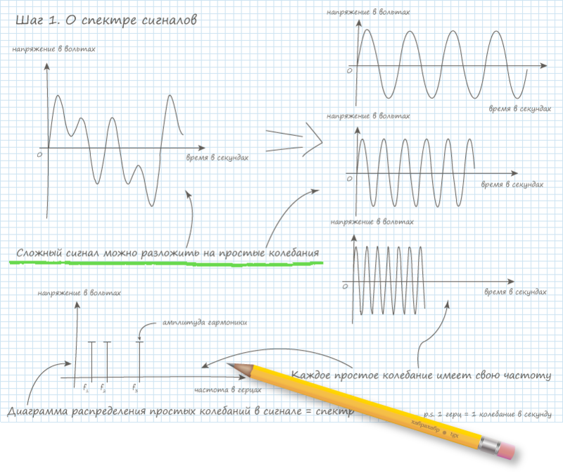
The signal observed on the oscilloscope (the previous picture) can be decomposed into elementary oscillations. Moreover, any physically observable signal can be subjected to such decomposition. Elementary oscillations are signals mathematically described by sine or cosine functions. In fact, sine and cosine are essentially the same signal, only slightly shifted in time.

If you start up all these elementary signals on the wire at the same time, then during the measurement you can see the initial “complex” signal.

Functions like sine are called harmonic. Therefore, they are often referred to as “complex” signal harmonics. Each signal has its own unique set of harmonics. This set of harmonics is called the signal spectrum . Spectral (harmonic) analysis deals with the study of signal harmonics.

Step 2. Mathematical waveform

Engineers and researchers use relatively simple mathematics to describe signals and their spectra. A complex signal is recorded as the sum of more simple ones, as shown in the figure:

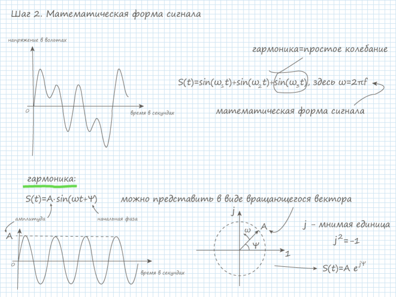
Each harmonic, as already mentioned, is a simple oscillation, described by a mathematical function sine. The coefficient in front of the sine is called “amplitude”, and the argument is called “phase”. Phase is the sum of two numbers. The first term is the product of time and the circular frequency, and the second term is the initial phase. Harmonics of the complex signal under consideration have a zero initial phase; this was chosen for clarity. In order not to confuse the usual phase with the initial one, it is called the “complete phase”. Explanations on the terms "phase", "initial phase", "amplitude", "cyclic (circular) frequency" and "function" can be found in textbooks in mathematics. I will only note that when the word “phase” occurs in literature, it is usually understood as a certain state, i.e. "Phase" = "state". In our case, the complete phase of the harmonic signal describes a state of the function at a given time. In other words, knowing the law of harmonic change (sine) and its current state (full phase), you can find out what the harmonic value is now.

Recording with sinuses is not always convenient. In engineering practice, they usually switch to the entry form in the exhibitor view. This has some advantages. More details can be found in the literature. It should be noted that when writing in the form of exponent complex numbers are used. The theory of these numbers is inextricably linked with the concept of imaginary unit. The visually exponential form can be represented as a rotating vector, as shown in the picture above. It rotates with a cyclic frequency in the plane, where real numbers are plotted along one axis, and imaginary numbers along the other. All this can also be read in more detail in the mathematical and engineering literature.

Step 3. Fourier Transform

In mathematics, there is a very important transformation that links the signal and its spectrum. It is called the Fourier transform . For clarity, you can look at the picture.

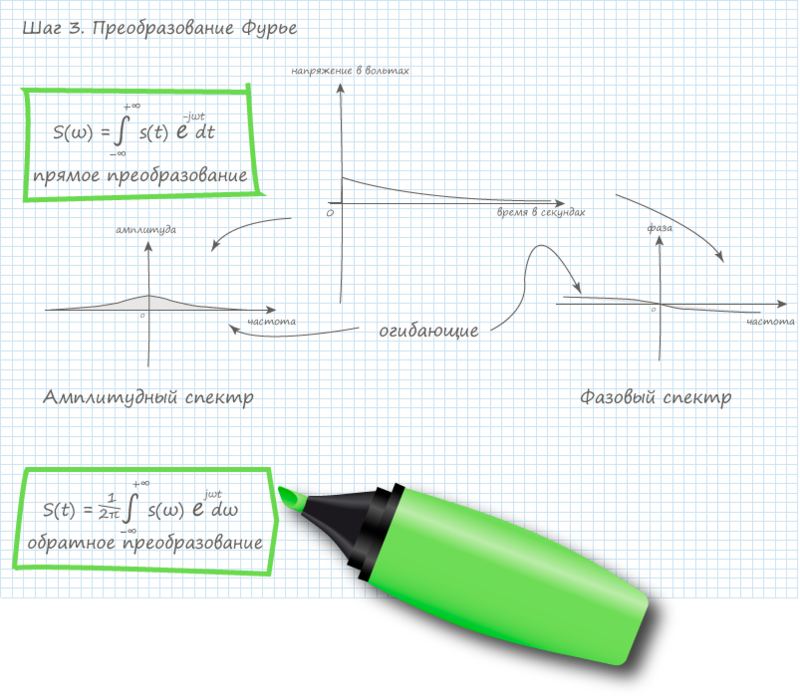
In the Fourier transform there are 2 formulas: in the picture they are circled with a marker. Forward conversion converts a signal into a spectrum, and the inverse converts a spectrum into a signal. In the formula, you need to substitute the functions that describe either the spectrum or the signal, depending on the type of conversion. About why formulas have just such a form can again be read in books on mathematics. There you can understand when you can apply the Fourier transform, and when you can not. And what to do if you can not apply, and the spectrum must be obtained. For most of the real-life signals, the Fourier transform is valid, but the remaining cases will not be considered.

After a direct transformation of the signal shown in the picture as a decaying exponent, we obtain its spectrum. In general, any spectrum is a complex number. Above mentioned numbers and the form of recording signals in the form of exponents. In this form, there are two signal parameters: amplitude and initial phase. If the signal is complex, then it consists of several harmonics, each harmonic has its own amplitude and its own phase. It's mathematically easy to count. In the exponential recording of the signal, instead of the usual amplitude and initial phase numbers, the functions of amplitude versus frequency and initial phase versus frequency are recorded. Such dependencies gives a direct Fourier transform on the output. As a result, the amplitude spectrum and the phase spectrum of the signal are selected. The picture above shows these spectra. They consist of a large number of harmonics, so drawing them is not clearly. Usually only envelopes are depicted.

Complex signals can be laid out not only on sines or cosines, or, by the way, if you notice, exhibitors. There are other classes of "elementary" functions, in the form of the sum of which you can represent a signal. All these functions within a class have a common property - “orthogonality”. Or in other words - perpendicularity. Thus, if we take two orthogonal functions and imagine that they are not functions, but vectors, then there will be an angle of 90 degrees between them. If you multiply these two functions, you get zero. This is not just zero, there is a certain meaning behind this zero: the mutual energy between orthogonal signals is zero, i.e. they do not interact with each other.

Step 4. Fast Fourier Transform

The technique has a sufficient number of techniques that produce analogue Fourier transform. There are even systems that do it instantly at the speed of light. However, in digital technology, where discrete signals are used, the use of analog transducers is often not appropriate. As a result, a mathematical algorithm that allows you to quickly obtain a signal spectrum has gained immense popularity. The algorithm is called the Fast Fourier Transform (FFT), its simplified diagram is shown in the figure below.

1. Fast Fourier transform works with discrete signals. A discrete signal is a set of numbers taken over a certain period of time from the values ​​of an analog signal.
2. The discretization of the signal is performed according to certain rules. This is a topic for another conversation. To whom it is interesting, you can search for articles or books on the subject of Kotelnikov (Shannon) theorem. If each number from a set of a discrete signal is represented as a binary code , then a digital signal is obtained. Ultimately, from an analog signal duration T is obtained an array of N numbers (points).
3. The task of the discrete Fourier transform is to obtain an array of spectrum numbers from an array of signal samples . These numbers are coefficients for orthogonal expansion functions, which were discussed above. The discrete form of the Fourier transform from analog is quite simple. The final view can be seen in the picture (at number 3).
4. From this moment begins the algorithm of the fast Fourier transform. The algorithm works best for arrays whose size is a multiple of a power of two. Therefore, if the number of reports is different from the power of two, then they are increased, rounded up, with the missing elements filled with zero values. The entire sequence is divided into two parts: even and odd readings. The lengths of the sequences obtained are N / 2.
5. Simple mathematical transformations show that for samples to N / 2, the formula shown in the figure (number 5) is valid.
6. For values ​​on the second half of the readings: from N / 2 to N, you can also go to a simple formula. It is obtained on the basis of the periodicity of the coefficients C. As a result, the complete formula for any coefficient C can be written as shown in the figure (numbered 6).
7. In this form, the algorithm gives some gain in speed. If the spectrum is received from the discrete signal “head-on” (formula number 3 in the figure), then this will require N multiplication operations by a complex number and N additions. And this is only to get one spectral coefficient, and there are a total of N. In the end, to get all the coefficients, you must perform N ² multiplications and N ² additions. If we use the expression obtained above (formula number 6 in the figure), then we need 2 (N / 2) ² + N multiplications. This is almost two times less. By splitting each sequence, up to two-element arrays, you can further reduce the number of calculations, as shown in the figure (number 7). This technique leads to approximately N log ₂ N multiplication operations. For example, for 1024 samples, the number of multiplication operations is reduced by 100 times! This greatly simplifies the application of Fourier transform in engineering.

Step 5. Modulation

Consider another complex signal on an oscilloscope .

This is an analog amplitude modulated signal. What is it about? If the task is to transmit information, for example, from the microphone in the headset to the phone "by air", then to solve it, you must first read the voice (sound) and then transfer it to the phone in some way. Now, similarly, tasks already have many elegant solutions that are optimal in one way or another parameter. For clarity, we can consider an example.

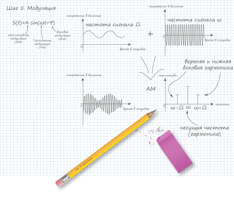
The figure briefly describes the essence of the signal modulation procedure. At its core, the concept of modulation is associated with a change in a parameter of one signal (high frequency) depending on another (low frequency). There are a diverse number of modulation schemes (types) that allow the signal to be transmitted best in a given situation, but it all comes down to a change in either the amplitude or the frequency or initial phase of the signal.

Low frequency signal carries information. For example, in our case, for simplicity, this is some kind of single-tone sound, i.e. simple signal. Depending on the amplitude of this signal, the envelope of the high-frequency signal changes. The high-frequency signal is called “carrier”, in the sense that it carries (carries) information. Sometimes it is possible to transmit an information signal without a modulation procedure. In reality, the signals are transmitted through some physical medium, and even in the conditions of interference. In order to successfully transmit the signal in this case, modulation is applied.

You can be convinced of the benefits of modulation by doing some calculations. It is known that the signals "through the air" are transmitted mainly with the help of electromagnetic fields in which waves propagate. Waves are emitted and received by antennas. Waves are characterized by "wavelength" . This value is the inverse of the frequency of the wave, which corresponds to the frequency of the transmitted signal. Obviously, the higher the frequency, the shorter the wavelength. Antenna sizes depend on the wavelengths with which they operate. Therefore, the larger the signal frequency, the smaller the antenna needed. For example, if you try to transfer the sound from the headset to the phone to the 5th octave 'To' (this is 4186.0 Hz), then the antenna size will be about 18 km long. And if you use the frequencies from the Bluetooth specification (about 2.4 GHz), then the antenna size will be only 3 cm. Of course, the estimates are estimated, but the result will make sure the modulation is useful.

As already mentioned, there are a large number of modulation schemes. However, digital modulation schemes are slightly different from analog, partially discussed above. Therefore, you should pay attention to them. As in analog circuits, it all comes down to a change in basically three parameters: frequency, phase, and amplitude, except that the parameters change in jumps. This kind of modulation is called "manipulation" (English shift key). The figure below shows the amplitude (ASK), frequency (FSK) and phase (PSK) patterns.

In modern communication systems, the QAM (quadrature) amplitude manipulation type has gained much popularity. The essence of which consists in the synthesis of a signal from the sum of two simple signals, the phase difference between which is 90 degrees (they are in quadrature). The amplitudes of these simple signals change discretely, which ultimately forms a signal with discrete variation of both amplitude and phase simultaneously. It is convenient to depict all possible states on the phase plane. In the figure above, such a plane is shown for modulating 16-QAM, i.e. 16 different states can be encoded with one QAM modulation symbol, which corresponds to 4-bits of information. By the way, based on such considerations - phase manipulation can be considered as a special case. For example, QPSK manipulation may be referred to as 4-QAM. Thus, changing the manipulation scheme can increase or decrease the speed of data flow. However, increasing the speed, you have to sacrifice noise immunity. In the various communication channels used "golden mean". Along with undeniable advantages, QAM has its drawbacks. The considered modulation schemes are often not used in their pure form. All this can be found in books on modern communication systems.

Step 6. Multiplexing

Telecommunications system developers face the constant challenge of a limited media resource, be it time, space, frequency, or code. Therefore, if you need to transfer multiple data streams for a single user or for several, you have to solve the problem of multiple access to the environment. , . (MAC).

. MIMO (. Multiple Input Multiple Output), . , , . « » - . . , .

FDM (Frequency Division Multiplexing). . .

, - , . , , .

TDM (Time Division Multiplexing). .

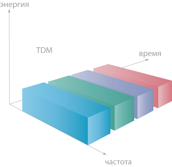
, . . TDM , , - () , . , TDM, GSM.

CDM (Code Division Multiplexing). .

- . . CDM , . , . . . .

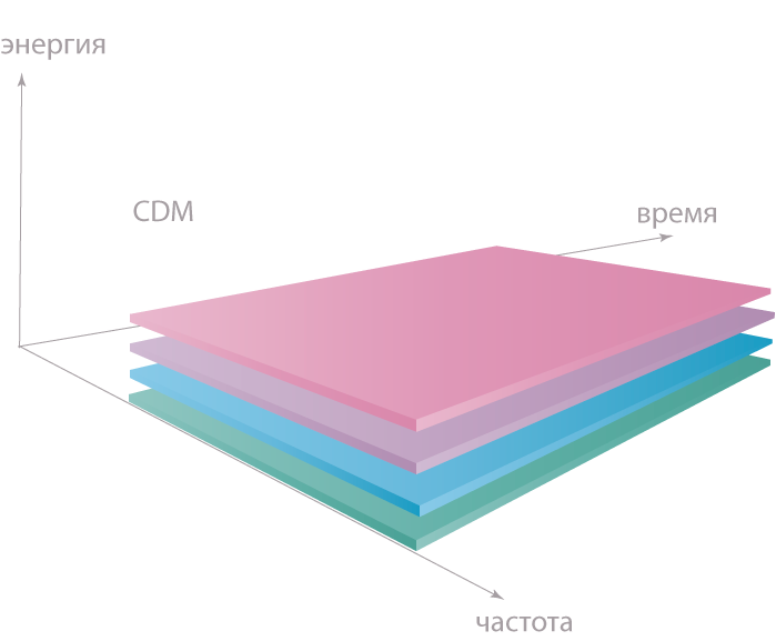
CDM. , CDM FMD FHSS (Frequency Hopping Spread Spectrum), TDM THSS (Time Hopping Spread Spectrum). , , CDM. , FHSS Bluetooth. CDM FDM , , OFDM.

, multiple access, FDMA, TDMA, CDMA, OFDMA .. .

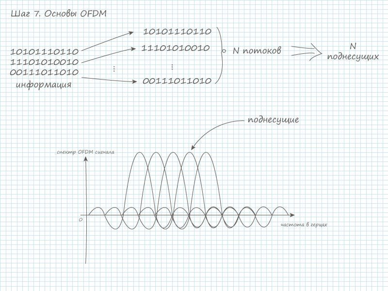
7. OFDM

OFDM ( ), . , .. N . . OFDM. . .

, OFDM — DVB . , , . OFDM , DVB-T .

1. DVB-T . . OFDM.
   
2. DVB-T 8 (7, 6 ). . OFDM .
   
   
   
3. OFDM . , .. , . , . 1/4, 1/8, 1/16 1/32 OFDM . .
   
   
   
   
   
   , () , , , . , . . , OFDM . .
4. , . . , OFDM , , QPSK, 16-QAM 64-QAM. , () .
5. OFDM , . . , . , (IFFT) . , . . OFDM.
   
   
   
   
   
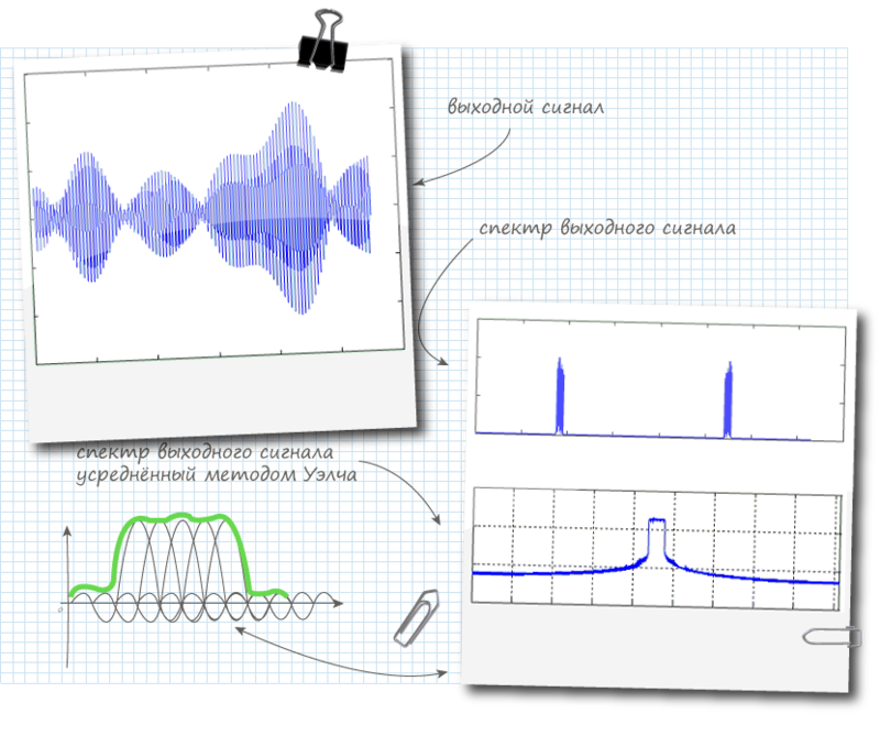
   , , QAM . , «» . .
6. , FFT/IFTT c , OFDM . , DVB-T 8k 2k, : 8000 2000 . 8192 (2 ¹³ ) 2048 (2 ¹¹ ), , 1705 6817, . OFDM DVB-T MatLAB :

1. %DVB-T 2K Transmission
2. % 8 MHz
3. %2K
4. clear all ;
5. close all ;
6. %DVB-T
7. Tu=224e-6; % OFDM
8. T=Tu/ 2048 ; %
9. G= 1 / 4 ; % 1/4, 1/8, 1/16, 1/32
10. delta=G*Tu; %
11. Ts=delta+Tu; % OFDM
12. Kmax= 1705 ; %
13. Kmin= 0 ;
14. FS= 4096 ; %IFFT/FFT
15. q= 10 ; %
16. fc=q* 1 /T; %
17. Rs= 4 *fc; %
18. t= 0 : 1 /Rs:Tu;
20. %
21. M=Kmax+ 1 ;
22. rand ( 'state' , 0 ) ;
23. a=- 1 + 2 * round ( rand ( M, 1 ) ) .' +i * ( - 1 + 2 * round ( rand ( M, 1 ) ) ) .';
24. A= length ( a ) ;
25. info= zeros ( FS, 1 ) ;
26. plot ( info ) ;
27. info ( 1 : ( A/ 2 ) ) = [ a ( 1 : ( A/ 2 ) ) .' ] ;
28. info ( ( FS- ( ( A/ 2 ) - 1 ) ) :FS ) = [ a ( ( ( A/ 2 ) + 1 ) :A ) .' ] ;
30. %
31. carriers=FS.* ifft ( info,FS ) ;
32. tt= 0 :T/ 2 :Tu;
33. figure ( 1 ) ;
34. subplot ( 211 ) ;
35. stem ( tt ( 1 : 20 ) , real ( carriers ( 1 : 20 ) ) ) ; %
36. subplot ( 212 ) ;
37. stem ( tt ( 1 : 20 ) , imag ( carriers ( 1 : 20 ) ) ) ; %
38. figure ( 2 ) ;
39. f= ( 2 /T ) * ( 1 : ( FS ) ) / ( FS ) ;
40. subplot ( 211 ) ;
41. plot ( f, abs ( fft ( carriers,FS ) ) /FS ) ;
42. subplot ( 212 ) ;
43. pwelch ( carriers, [ ] , [ ] , [ ] , 2 /T ) ;
45. %
46. L = length ( carriers ) ;
47. chips = [ carriers.';zeros ( ( 2 *q ) - 1 ,L ) ] ; %
48. p= 1 /Rs: 1 /Rs:T/ 2 ;
49. g= ones ( length ( p ) , 1 ) ;
50. figure ( 3 ) ;
51. stem ( p,g ) ;
53. dummy= conv ( g,chips ( : ) ) ; %
54. u= [ dummy ( 1 : length ( t ) ) ] ; %
55. figure ( 4 ) ;
56. subplot ( 211 ) ;
57. plot ( t ( 1 : 400 ) , real ( u ( 1 : 400 ) ) ) ;
58. subplot ( 212 ) ;
59. plot ( t ( 1 : 400 ) , imag ( u ( 1 : 400 ) ) ) ;
61. figure ( 5 ) ;
62. ff= ( Rs ) * ( 1 : ( q*FS ) ) / ( q*FS ) ;
63. subplot ( 211 ) ;
64. plot ( ff, abs ( fft ( u,q*FS ) ) /FS ) ;
65. subplot ( 212 ) ;
66. pwelch ( u, [ ] , [ ] , [ ] ,Rs ) ;
68. [ b,a ] = butter ( 13 , 1 / 20 ) ; %
69. [ H,F ] = FREQZ ( b,a,FS,Rs ) ;
70. figure ( 6 ) ;
71. plot ( F, 20 * log10 ( abs ( H ) ) ) ;
72. uoft = filter ( b,a,u ) ; %
74. figure ( 7 ) ;
75. subplot ( 211 ) ;
76. plot ( t ( 80 : 480 ) , real ( uoft ( 80 : 480 ) ) ) ;
77. subplot ( 212 ) ;
78. plot ( t ( 80 : 480 ) , imag ( uoft ( 80 : 480 ) ) ) ;
80. figure ( 8 ) ;
81. subplot ( 211 ) ;
82. plot ( ff, abs ( fft ( uoft,q*FS ) ) /FS ) ;
83. subplot ( 212 ) ;
84. pwelch ( uoft, [ ] , [ ] , [ ] ,Rs ) ;
86. %Upconverter
87. s_tilde= ( uoft.' ) .* exp ( 1i * 2 * pi *fc*t ) ;
88. s= real ( s_tilde ) ;
89. figure ( 9 ) ;
90. plot ( t ( 80 : 480 ) ,s ( 80 : 480 ) ) ;
91. figure ( 10 ) ;
92. subplot ( 211 ) ;
93. %plot(ff,abs(fft(((real(uoft).').*cos(2*pi*fc*t)),q*FS))/FS);
94. %plot(ff,abs(fft(((imag(uoft).').*sin(2*pi*fc*t)),q*FS))/FS);
95. plot ( ff, abs ( fft ( s,q*FS ) ) /FS ) ;
96. subplot ( 212 ) ;
97. %pwelch(((real(uoft).').*cos(2*pi*fc*t)),[],[],[],Rs);
98. %pwelch(((imag(uoft).').*sin(2*pi*fc*t)),[],[],[],Rs);
99. pwelch ( s, [ ] , [ ] , [ ] ,Rs ) ;

Guillermo Acosta. :

8. OFDM

OFDM, .

1. COFDM (Coded OFDM). OFDM , . DVB-T , OFDM.
2. Flash OFDM (Fast low-latency access with seamless handoff OFDM). Flarion Technologies . . . , .
3. OFDMA . . OFDM .
4. VOFDM (Vector OFDM). Cisco Systems . MIMO. MIMO-OFDM.
5. WOFDM (Wideband OFDM). Shirokoloposnaya modification OFDM developed Wi-Inc the LAN . In the modification is achieved by increasing the bandwidth and noise immunity. The main difference in the larger frequency distance between the carriers.

Step 9. Conclusion

OFDM. , , , . OFDM, , , , . .

10.

1. OFDM-Based Broadband Wireless Networks. Design and Optimization. Hui Liu and Guoqing Li
2. Multi-Carrier and Spread Spectrum Systems. From OFDM and MC-CDMA to LTE and WiMAX. K. Fazel, S. Kaiser
3. OFDM. Concepts for Future Communication Systems. Hermann Rohling
4. . .
5. . . .
6. . . .
7. . . .
8. . . .
9. . .., ..
10. MATLAB ( ViruScD ).
11. ( eucariot ).