You need to know your tool in person: an overview of the most frequently used data structures

Some time ago I went to an interview in one rather large and respected company. The interview went well and I liked it, and I hope the people who conducted it. But the next day, during the debriefing process, I found that during the interview the answer to at least one question was incorrect.



Question: Why does the search in python dict on large amounts of data faster than iterating over an indexed array?



Answer: Dict stores key hashes. Every time when we search for dict value by key, we first calculate its hash, and then (suddenly), we perform a binary search. Thus, the complexity is O (lg (N))!

')

In fact, there is no binary search here. And the complexity of the algorithm is not O (lg (N)), but Amort. O (1) - since dict python is based on a structure called Hash Table.



The reason for the wrong answer was that I did not bother to thoroughly study the structures that underlie the work with the collections of my favorite language . However, according to the results of a survey of several familiar developers, it turned out that this is not only my problem, many people do not even think at all how the collections in their favorite PL work. But we use them every day and not just once. So the idea of ​​this article was born.





A few words about the classification of structures in the article. If you study the sources that are listed in the list of information used, you will notice that the classification in this article does not match the classification in any of the sources (in some sources it is not at all). This is due to the fact that it seemed to me more expedient to view structures in the context of their use. For example, an associative array in PHP / Python / C ++ or a list in .Net / Python.



So let's go.

1. Array - it is an indexed array.

Array is a fixed-size collection consisting of elements of the same type.



Interface:

• get_element_at (i): O (1) complexity
• set_element_at (i, value): O (1) complexity

An array search is performed by enumerating elements by indices => O (N) complexity.



Why is the access time to an item by index constantly? The array consists of elements of the same type, has a fixed size and is located in a continuous memory area => to get the j-th element of the array, we just need to take a pointer to the beginning of the array and add to it the size of the element multiplied by its index. The result of this simple calculation will indicate exactly the desired element of the array.

*aj = beginPointer + elementSize*j-1





Examples:

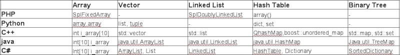
/++: int i_array[10];

java/C#: int[10] i_array;

Python: array.array

php: SplFixedArray



2. List (list).

A List is a list of elements of an arbitrary type of variable length (that is, we can at any time add an element to the list or delete it). The list allows you to iterate over the items, get items by index, as well as add and delete items. The implementations of the List are possible different, the main ones are (Single / Bidirectional) Linked List and Vector. Classic List provides the ability to work with it directly and through an iterator, the interfaces of both classes will be discussed below.



Interface List:

• prepend (item): Add an item to the top of the list.
• append (item): Add an item to the end of the list.
• insert_after (List Iterator, item): Add an item after the current one.
• remove_firts (): Remove the first item.
• remove_after (List Iterator): Remove the item after the current one.
• is_empty (): Is the List empty.
• get_size (): Returns the size of the list.
• get_nth (n): Return the nth item.
• set_nth (n, value): Set the value of the nth element.

List Iterator Interface:

• get_value (): get the value of the current element.
• set_value (): set the value of the current element.
• move_next (): move to the next element.
• equal (List Iterator): checks if another iterator refers to the same list item.

It should be noted that in some (mainly interpreted) programming languages, these two interfaces are “glued together” and “cropped”. For example, in python, an object of type list can be iterated, but you can also get a value from it by referring directly to the index.



Let us turn to the implementations of the list.

2.1 Single Linked List

A unidirectional linked list (a simply linked list) is a chain of containers. Each container contains within itself a link to the item and a link to the next container, so we can always move forward along the simply linked list and can always get the value of the current item. Containers can be located in the memory as they please => adding a new element to the simply linked list is trivial.



Cost of operations:

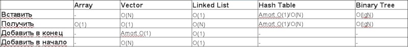
• prepend: o (1)
• insert_after: O (1)
• remove_first / remove_after: O (1)
• get_nth / set_nth: O (N)

Examples:

/++: std::list //Bidirectional Linked List

Java: java.util.LinkedList

c#: System.Collection.Generic.LinkedList //Bidirectional Linked List

php: SplDoublyLinkedList // Bidirectional Linked List





We will not consider the Bidirectional Linked List in detail, the whole difference between it and the Single Linked List is that the containers have a link not only to the next one, but also to the previous container, which allows you to move through the list not only forward, but also backward.

2.2 Vector

Vector is a List implementation through an extension of an indexed array.



Cost of operations:

• prepend: O (n)
• append: Amort.O (1)
• insert_after: O (N)
• remove_first / remove_after: O (1)
• get_nth / set_nth: O (1)

Obviously, the main advantage of Vector'a - quick access to the elements of the index, inherited them from the usual indexed array. It is also simple to iterate a Vector; it is enough to increment a certain counter by one and access it by index. But for the speed of access to the elements have to pay the time of their addition. In order to insert an element in the middle of Vector'a (insert-after), you must copy all elements between the current position of the iterator and the end of the array, as a result, the access time is on average O (N). The same with the removal of the element in the middle of the array, and with the addition of the element at the beginning of the array. Adding an element to the end of the array can be done in O (1), but it may not be - if you again need to copy the array to a new one, it is said that adding an element to the end of the Vector occurs in Amort. O (1).



Examples:

/++: std::vector

Java: java.util.ArrayList

C#: System.Collections.ArrayList, System.Collections.List

Python: list



3. Associative array (Dictionary / Map)

Collection key pairs => value. Elements (values) can be of any type, keys are usually only strings / integers, but in some implementations the range of objects that can be used as a key can be wider. The size of an associative array can be changed by adding / removing elements.



Interface:

• add (key, value) - add item
• reassign (key, value) - replace element
• delete (key) - delete item
• lookup (key) - find item

There are two main implementations of the Associative array: HashMap and Binary Tree.

3.1 Hash Table

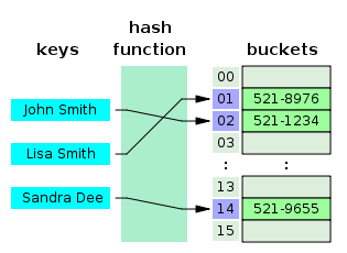
As the name suggests, hashes are used here. The mechanics of the Hash Table work are as follows: it is based on the same indexed array, in which the index is the value of the hash from the key, and the value is a reference to the object containing the key and the stored item (bucket). When an item is added, the hash function calculates the hash from the key and stores a reference to the added item in the array cell with the corresponding index. To get access to the element, we again take the hash from the key and, working just like with a regular array, we get a reference to the element.



An inquisitive reader may notice some problems that are characteristic of the implementation of this SD.

• If the hash of the key is equal, for example, 1928132371827612 - this will mean that we need to have an array of the appropriate size? And if we have only 2 elements in it?
• And if we have hashes from two different keys match?

These two problems are connected: it is obvious that we cannot calculate long hashes, if we want to store a small number of elements, this will lead to unreasonable memory costs, because the hash function usually looks something like this:

index = f(key, arrayLength)





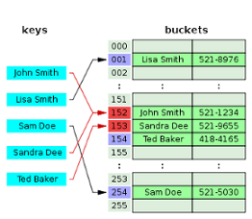
That is, besides the key value, it also receives the current size of the array, this is necessary to determine the length of the hash: if we store only 3 elements, there is no point in making a hash 32 bits long. The reverse side of this behavior hash function - the possibility of collisions. Collisions are actually characteristic of the Hash Table, and there are two methods for resolving them:



Chaining:



Each cell of the array H is a pointer to a linked list (chain) of key-value pairs corresponding to the same key hash value. Collisions simply lead to the fact that there are chains with a length of more than one element.



Open addressing:



The H-key pairs themselves are stored in the array. The element insertion algorithm checks the cells of the array H in a certain order until the first free cell is found, in which the new element will be written. This order is calculated on the fly, which saves memory for pointers required in chained hash tables.





Cost of operations:

• add: Amort.O (1) / O (N)
• reasign: Amort.O (1) / O (N)
• delete: Amort.O (1) / O (N)
• lookup: Amort.O (1) / O (N)

Here, the first value is the average complexity, the second is the complexity of the operation at worst. This difference is due to the following: when adding an element, if the array is full, you may need to rebuild the entire Hash Table. When searching for an element it may turn out that we stumble upon a long chain of collisions, and again we will have to sort through all the elements.



Examples:

c++: QHash boost::unordered_map/boost::unordered_set (by NickLion )

java: java.util.HashMap<K,V>

c#: System.Collections.Hashtable, System.Collections.Dictionary<K, V>

python: dict

php: array()



3.2 Binary Tree

In fact, not just a Binary Tree, but a Self-balancing Binary Tree. Moreover, it should be noted that there are several different trees that can be used to implement the Associative array: red-black tree, AVL-tree, etc. We will not consider each of these trees in detail, since this is possibly a topic of another, separate article, and maybe several (if you study trees very carefully). We describe only the general principles.



Definition: a binary tree is a tree data structure in which each node has no more than two descendants (children). As a rule, the first is called the parent node, and children are called left and right heirs. If the node has no heirs - it is called a leaf node.



For example, let's take a binary search tree: each node is a container containing three elements: data is the actual data bound (data contains both the element itself and the key value), left is a link to the left lower node and right - link to the right lower node. In this case, the following rule is executed: key [left [X]] <key [X] ≤ key [right [X]] —that is, the data keys of the parent node are larger than the data keys of the left son and weakly less than the data keys of the right one. When searching for an element, we go around the tree, each time comparing the value of our key with the key of the current node, and, by comparison, determining which way to go. It is easy to calculate that the complexity of such a search is stable O (lgN). When adding a new node, we perform a generally similar procedure until we find where to insert a new element. True, it should be noted that such trees still need to be balanced - but this we will already omit. An inquisitive reader will find the necessary information by examining the list of sources.



Cost of operations:

• add: Amort.O (lgN)
• reasign: Amort.O (lgN)
• delete: Amort.O (lgN)
• lookup: Amort.O (lgN)

Examples:

c++: std::map, std::set

java: java.util.TreeMap<K,V>, java.util.Map<K,V> -

c#: :( SortedDictionary(by NickLion )

python: -

php: -



4. Set (Set).

Immutable set of elements. The set is defined once - at creation, and further provides access to elements only for reading. The set cannot be expanded, nor can the elements be removed from it or the element of the set be changed. As a base for the implementation of this collection is usually used Hash Table - a description of which, see. Above.



A set is simply a realization of the abstraction of a mathematical set, i.e. set of unique distinguishable elements. ( spn . danilI )

Examples:

c++: std::set

java: java.util.Set

C#: System.Collections.HashSet

python: set/frozenset





Comparative characteristics of data structures:





Data structures in various programming languages:

References:

Data Structures (en)

Data Structures (rus)

Binary search tree (en)

Binary Search Tree (rus)



Also the author looked into the PHP source and read the dock for STL .



Upd. Yes, there is a regular indexed array in array (array.array). Thanks enchantner. With the amendment, the type is not necessarily numeric, the type can be specified.



Upd. Made a lot of corrections in the text. idemura , zibada , tzlom , SiGMan , freeOne , Slaffko , korvindest , Laplace , enchantner thanks for the edits!



Upd.

From zibada comments:

Yes, that’s just because of the lack of a description of the Map iteration from the article, it’s not at all clear why it would seem that trees are needed when there are hashes. (O (logN) versus O (1)).



They are needed in order to list the Map (or Set) elements you want:

- in any non-guaranteed order (HashMap, embedded hashes in some scripting languages);

- in the order of addition (LinkedHashMap, embedded hashes in some other scripting languages);

- in ascending order of keys + the ability to iterate only the keys in the specified range.



But for the latter case, an alternative to trees is just a complete sorting of the entire collection after each change or before a request.

What is long and sad for large collections, but it works for small ones - that is why trees are not specifically built into scripting languages.