Checkout right
The problem with most of today's programs, such as Excel or Numbers - they give a disgusting set of typical graphs, from which the user needs to choose the right one. But how can one choose a suitable and good one, if one needs to complete about a dozen difficult gestures, each of which can be dealt with in 5-10 minutes ...
Therefore, today's article will be devoted to how correctly and clearly you need to draw up graphics in presentations.
Start over.
Here, the most common schedule, which is created in a second, by pressing 2 buttons in Excel. Yes, beauty is indescribable, that the eye does not tear. But is this beauty so important when you need to give a clear and understandable idea to all those who have gathered about what is happening with the company's budget? Someone will be able to unequivocally say what happens, for example, in the month of June? Is the company at a loss? Or maybe the other way around is not so bad? To answer this question you need to connect a good spatial imagination and good luck. And then someone will be able to answer: “In June, the budget has finally exceeded our expenses!” .
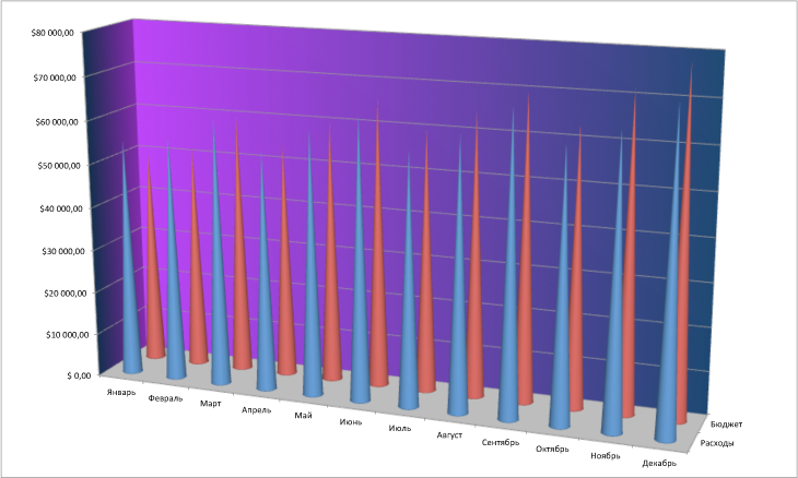
It's great that at least someone could figure it out, but not everyone can do it. Therefore, we will have to greatly modify this graph to make it understandable even for an unprepared person who is used to working only with digital tables and trusting only numbers.
')
First you need to remove completely unnecessary 3D effect, which, as you already understood, only introduces huge distortions in the display of data.
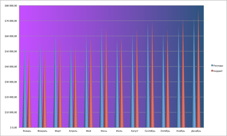
This seemingly insignificant change in the schedule has already become much clearer, but still far from ideal.
Now the most important thing is to remove this “flashy” background, which is very confusing because of its gorgeous coloring.
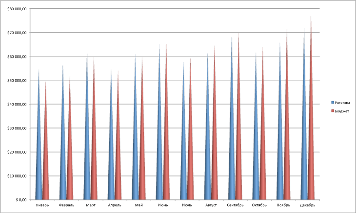
The correct perception of the chart still complicates the shape of the bars (vertical pyramids), which have a taper. Replace them with a good old histogram with ordinary bars.

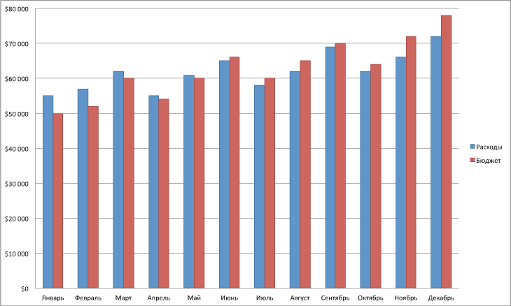
Now is the time to start “cleaning” the graph itself from excessive visual garbage, which does not carry any semantic load. Remove the "fence" from risok on the vertical and horizontal axes.
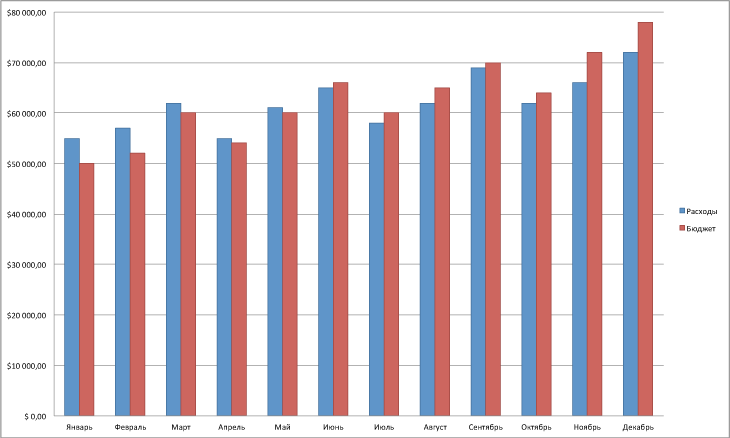
The schedule began to look at least decently. Now you need to understand the signatures on the axes. Let's start with the most voluminous axis in terms of the number of digits - the vertical currency. As a minimum, 2 decimal places can be removed from numerical values, especially since there are zeroes everywhere. In addition, we will slightly increase in size all the signatures for their better readability.
The name of the vertical axis is better to make a single word, and not to denote each new digit with the $ symbol.
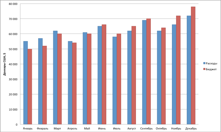
Red and blue (even muffled) - not the best combination of colors for comparison. When a graph compares 2 values, then by default only one can be the dominant (main) value, and not both. In our case, the most interesting value is “Consumption”. Therefore, it also needs to be highlighted in color, and the “Budget” value should be made in gray so that it does not stand out so much. In addition, we move the name of the vertical axis and the legend to the top of the whole diagram.
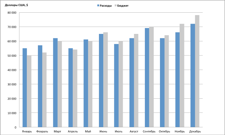
But, strictly speaking, a histogram is not the best kind of graph for time comparisons, which we produce here. To do this, use the usual linear graph with a curve that reflects the dynamics of a change in a particular value over time.
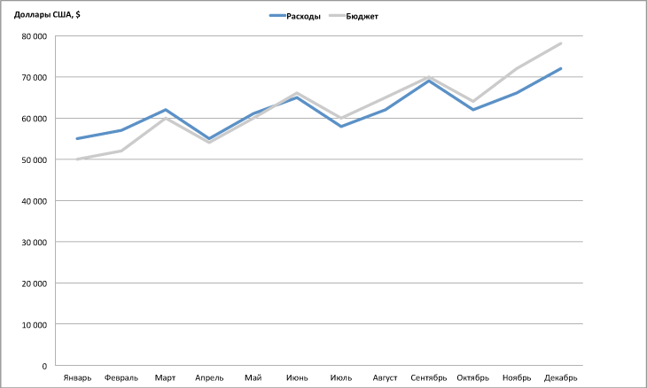
Most of the graphics remained untapped due to the previously selected scale. Therefore, we scale the graph to the entire available area.
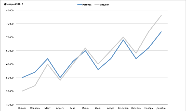
In principle, even now the graph has become 5 times more readable and clearer than the initial one. However, when there are not very many curves displayed on the graph, then the captions should be made right next to them and not the legend, which is not convenient to work with.

This graphic is great for displaying it on a projector. But what if it should be printed on a printer? And the printer also turned out to be black and white. In this case, it is necessary to replace the primary colors of the graphs with gradients of gray.

And now, if we recall the main task of the schedule, which I wrote at the very beginning: “... you need to give a clear and understandable idea to all those who have gathered about what is happening with the company's budget ...” . But 2 graphics do not give a definite answer to this question. Yes, we see that at the beginning of the summer the company's budget exceeded its expenses, but in order to understand by how much, you need to carry out mathematical calculations in your head that will prove to be inaccurate. Therefore, it is necessary to add both graphs in order to visualize this change.

Now, for even more understanding, let's replace cash equivalents by%, thus making our schedule even more expressive.

And in conclusion, look again at how the initial schedule has changed and how much its understanding has improved.

The difference is visible :)
PS - I didn’t describe how certain transformations are carried out in Excel, because it seems to me to be superfluous. However, if someone does not know how to make the given examples - write, I will.
Therefore, today's article will be devoted to how correctly and clearly you need to draw up graphics in presentations.
Start over.
Here, the most common schedule, which is created in a second, by pressing 2 buttons in Excel. Yes, beauty is indescribable, that the eye does not tear. But is this beauty so important when you need to give a clear and understandable idea to all those who have gathered about what is happening with the company's budget? Someone will be able to unequivocally say what happens, for example, in the month of June? Is the company at a loss? Or maybe the other way around is not so bad? To answer this question you need to connect a good spatial imagination and good luck. And then someone will be able to answer: “In June, the budget has finally exceeded our expenses!” .
It's great that at least someone could figure it out, but not everyone can do it. Therefore, we will have to greatly modify this graph to make it understandable even for an unprepared person who is used to working only with digital tables and trusting only numbers.
')
First you need to remove completely unnecessary 3D effect, which, as you already understood, only introduces huge distortions in the display of data.
This seemingly insignificant change in the schedule has already become much clearer, but still far from ideal.
Now the most important thing is to remove this “flashy” background, which is very confusing because of its gorgeous coloring.
The correct perception of the chart still complicates the shape of the bars (vertical pyramids), which have a taper. Replace them with a good old histogram with ordinary bars.
Now is the time to start “cleaning” the graph itself from excessive visual garbage, which does not carry any semantic load. Remove the "fence" from risok on the vertical and horizontal axes.
The schedule began to look at least decently. Now you need to understand the signatures on the axes. Let's start with the most voluminous axis in terms of the number of digits - the vertical currency. As a minimum, 2 decimal places can be removed from numerical values, especially since there are zeroes everywhere. In addition, we will slightly increase in size all the signatures for their better readability.
The name of the vertical axis is better to make a single word, and not to denote each new digit with the $ symbol.
Red and blue (even muffled) - not the best combination of colors for comparison. When a graph compares 2 values, then by default only one can be the dominant (main) value, and not both. In our case, the most interesting value is “Consumption”. Therefore, it also needs to be highlighted in color, and the “Budget” value should be made in gray so that it does not stand out so much. In addition, we move the name of the vertical axis and the legend to the top of the whole diagram.
But, strictly speaking, a histogram is not the best kind of graph for time comparisons, which we produce here. To do this, use the usual linear graph with a curve that reflects the dynamics of a change in a particular value over time.
Most of the graphics remained untapped due to the previously selected scale. Therefore, we scale the graph to the entire available area.
In principle, even now the graph has become 5 times more readable and clearer than the initial one. However, when there are not very many curves displayed on the graph, then the captions should be made right next to them and not the legend, which is not convenient to work with.
This graphic is great for displaying it on a projector. But what if it should be printed on a printer? And the printer also turned out to be black and white. In this case, it is necessary to replace the primary colors of the graphs with gradients of gray.
And now, if we recall the main task of the schedule, which I wrote at the very beginning: “... you need to give a clear and understandable idea to all those who have gathered about what is happening with the company's budget ...” . But 2 graphics do not give a definite answer to this question. Yes, we see that at the beginning of the summer the company's budget exceeded its expenses, but in order to understand by how much, you need to carry out mathematical calculations in your head that will prove to be inaccurate. Therefore, it is necessary to add both graphs in order to visualize this change.
Now, for even more understanding, let's replace cash equivalents by%, thus making our schedule even more expressive.
And in conclusion, look again at how the initial schedule has changed and how much its understanding has improved.
The difference is visible :)
PS - I didn’t describe how certain transformations are carried out in Excel, because it seems to me to be superfluous. However, if someone does not know how to make the given examples - write, I will.
Source: https://habr.com/ru/post/122830/
All Articles