Odorless filtering and non-linear estimation *

* from English "Unscented filtering and nonlinear estimation" (by Google Translator )
At the request of dmitriyn decided to publish his vision on the so-called "Unscented Kalman filter", which is the extension of Kalman linear filtering in the case when the dynamic and observation equations of the system are non-linear and cannot be adequately linearized.
As the name of this filtering method “kosher” is readily translated into Russian, I do not know yet what is reflected in the title of the article, so I decided to just copy-paste a rather amusing, in my opinion, machine translation. Another fun version of the translation is the insensitive filter .

UPD : Added a comment to the section "UT APPLICATION"

INTRODUCTION

In a previous article on linear Kalman filtering, one of the possible approaches to the synthesis of FC for the case of a linearized simplified mathematical model of a dynamic system was described. The Kalman filter described there is sometimes referred to in literature as “conventional Kalman Filter” [ 2 ]. This name he received, because gives the smallest root-mean-square error only if several hypotheses (conventions) are observed - for example, the noise is white and distributed according to the normal law, the expectation of the noise is zero, there are no correlations between the noise and the cross-links between the phase coordinates. These restrictions are quite serious and in practice often hypotheses are violated. There are techniques to circumvent these limitations (for example, adding coordinates to a phase vector filter for a colored noise generator and entering a fictitious perturbation for “biased” noise). All of them lead to an increase in computational complexity (the dimension of the problem grows) and difficulties in the synthesis of a filter that is resistant to violation of conventions.
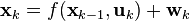
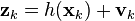
There is also an “Extended Kalman filter” [ 1 ], which is similar in its structure to the linear version, differing in that the equations of dynamics and observations contain non-linear (power, trigonometric, etc.) functions from the phase coordinates (see equations below). This difference also implies the existence of cross-links between phase coordinates (for example, the product of two coordinates).



')
When using EKF, it is necessary to calculate the Jacobian, a matrix of partial derivatives of the phase coordinates, at each iteration step. Because of this, computational complexity greatly increases and the question of the stability of discretized differential equations becomes even more acute. In essence, EKF realizes in itself a linearization layer of a nonlinear dynamical system. This is the main reason why EKF may be ineffective. The use of a strongly non-linear model of a dynamic system leads to a very poor conditionality of the problem, i.e. small error of the parameters of the mat. models will lead to large computational errors. As a result, the algorithm will lose robustness (error tolerance).

The unscented Kalman filter (UKF) [ 3 ] uses a different approach ("unscented transform"). According to Wikipedia, this approach implies the choice of a certain minimum set of samples (sigma points) for the data of expectation and covariance of the desired vector with random interference superimposed on it. Nonlinear prediction functions are constructed by sigma points, which are then used to compute the crosscovariance matrix (the core of the Kalman filtering algorithm).
After writing the last paragraph I personally had more questions. Like St. Augustine, who knew what time was, until he was asked about the time. Below I will try to explain to myself and you, dear readers, the essence of the considered method of nonlinear filtering.

UNSCENTED TRANSFORM

Perhaps I'll start with a more detailed description of the two main problems of the linear Kalman filter (FC) and the nonlinear (extended, EKF). The first problem is interference conventions. As written above, the linear FC assumes that the noises are “white” and are distributed according to the normal law. If the noise is “colored”, then we must synthesize a digital shaping filter, by passing “white” noise through which we will receive noise with a spectral characteristic equivalent (ideally) or close to the existing de facto. The phase vector of this filter is added to the phase vector FC. This in turn increases the dimension of the problem. Suppose that this problem is not too serious. But there is a second - the problem of nonlinearity of the mathematical model. In consequence of non-linearity, we must implement an approximator that allows linearizing the non-linear matrix function (see “h” in the equation above) and thus provide the opportunity to separate the variables. Variables must be separated so that it is possible to make equations for the components of the phase vector. In the EKF, linearization is performed by calculating the Jacobian, i.e. For each equation in “h”, partial derivatives are calculated for each of the phase variables. By itself, this operation is already a problem - a large amount of computation. In addition, to calculate the Jacobian, a Taylor (multidimensional) series expansion is used:



In this case, only the first member of the series is taken, and the rest are assumed to be negligible. Thus, using this linearization, we obtain an expression of the form:


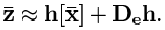
In this equation, “De” is the operator for calculating the total differential of the matrix function.

If the nonlinearity of the mathematical model is small (the model is almost linear), this statement can be considered true. However, in practice, the nonlinearities of the model are such that they do not allow rejection of the expansion terms of the second and / or higher orders of smallness. In such cases, the linearization in the EKF generates a computational error, which cannot be neglected. In some, particular cases, it is possible to do without decomposition into a Taylor series, but these are particular solutions that are rigidly tied to one specific object. There is also a solution that cuts the Taylor series to a member of the second order of smallness [6]. It involves the calculation of the Hessian - the second order derivative tensor. Just please do not make me chew what it is. Awareness of the fact that this makes EKF even more difficult and complicates its implementation is enough.
So, FC can be applied to a nonlinear model of an object if there is a certain transformation known that allows to project the current value of the phase vector (to make a “nonlinear” forecast) for the next iteration step. If this (adequate) transformation is unknown, then we use EKF with its, often also inadequate, linearization and a very large computational load. Thus, we need a method that allows one to dispense with the linearization used in the EKF, and which does not have more computational complexity compared to the EKF. This method is the “Unscented Transformation” (UT, do not further confuse this abbreviation with a computer game).

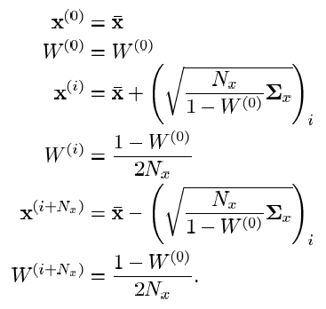
The main idea of ​​UT is to collect more frags in the intuitive assumption that it is much easier to approximate the probability distribution function of a random variable with a nonzero expectation (which is our phase vector - random interference is imposed on it) than to approximate some arbitrary nonlinear transformation function. This technique involves the selection of a set of points (sigma points) in the parameter space (phase coordinates), which characterizes with sufficient accuracy the statistical characteristics (expectation, dispersion and other higher-order moment characteristics) of the desired random vector (in our case, the phase vector with superimposed by the noise vector). To select these points, the following expressions are used:


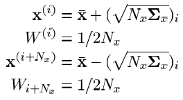
In these expressions, " Nx " is the dimension of the desired phase vector; " i " is the index of the sigma point (i = 1 .. Nx ); " Wi " is the weight of the ith sigma point;
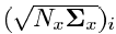- i- th column of the matrix square root of the covariance matrix of the initial non-linear transformation of the model multiplied by the dimension of the phase vector.

It should be noted that this is not the only option for a set of sigma points. The above expressions uniquely characterize the distribution statistics only for the first and second moments (expectation and variance). UT, characterizing the statistics of the distribution of the desired vector to moments of higher orders, differ in the number of sigma points (generally speaking, their number will not necessarily be greater than for the expressions above) and the choice of weights. For simplicity, I will omit the details. I will cite only as an example the expressions for UT, which take into account the higher orders of the moments of the statistics of the distribution of the phase vector:


In principle, about UT itself, in short, everything. Why it is needed and how it is used in the UKF is written below. Here it is necessary to make a reservation about the moment characteristics of high orders. What it is? An intuitive analogy is the position, speed, and acceleration of a moving body. If we consider the position as a moment of the first order, then the speed will be the second moment (rate of change of position), and acceleration - the third (speed of change of speed). You can calculate the derivative of acceleration - we get the fourth moment. But does it have a practical meaning? Similarly, with the moment characteristics in statistics - in most cases, the expectation and variance are sufficient. From the statistical accuracy of UT, i.e. on the method of choosing sigma points, the filtering efficiency depends, but probably not so much that for most practical problems there was a need to take into account the moment characteristics of high orders.

APPLICATION UT

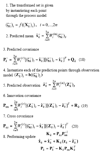
As mentioned above, UT is a method to get rid of the linearization procedure in non-linear stochastic estimation. So far we have only learned that with the help of UT it is possible to pick up a set of points that quite accurately characterize the statistics of the desired vector (phase vector). What does this give us? The key point in Kalman filtering is the calculation of the crosscovariance matrix (see the “Kk” matrix in the previous article ). This matrix in a linear FC is calculated as a solution of the matrix Riccati equation. In the case of a nonlinear mat. model of the system, this procedure is very complicated. UT makes it possible to obtain an alternate cross-crossing matrix. Below is a step-by-step filtering procedure using the UT method.

1. Find the statistical parameters of the desired vector (phase vector or vector of observation - the vector of the output signals of the sensors). The obtained statistical characteristics can be considered constant or updated in real time.
2. According to the obtained statistical data we calculate the set of sigma points.
3. We skip these points through the original non-linear mat. dynamic process model:
   
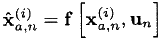
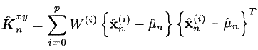
4. We calculate the forecast of expectation and covariance:
   
   
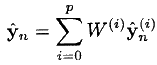
5. We skip the points obtained at the third step through the observation model (in the general case also non-linear):
   
6. We calculate the forecast of observation (in the form of a weighted average of the values ​​in the previous step):
   
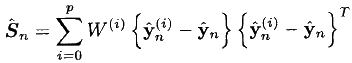
7. Calculate the covariance of the observation:
   
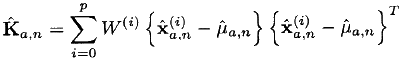
8. Find the desired cross-sharing matrix:
   
9. Finally, we use the standard FC expressions:
   

The last block of expressions is copied from article [3] as is. In my opinion something is wrong in it. It is not clear where the “yn” without a cap and the cross-crossing matrix with unmarked signs are taken from. But it does not matter. About the "standard expressions FC" I already wrote. It is only necessary to substitute in them the matrix gain found by UT Kalmans (also known as the crosscovariance matrix) and calculate the corrected estimate of the phase vector.
Another remark about the phase vector. In the expressions above, there is a phase vector with the index “a” (Xa, n) - this is the phase vector supplemented (augmented) with coordinates for process noise and observation. At the very beginning I wrote that there is such a technique for circumventing the limitation on the spectral characteristic of interference. So, in the expressions above, somehow, the transition from augmented vectors to ordinary ones was made in a quiet way (there is also a simple and complementary expectation of mu).

CONCLUSION

So, using UT, we were able to calculate the prediction of the phase vector and the crosscovariance matrix without linearization. Substituting their values ​​in the standard expressions for the correction phase of the prediction FC (see "Measurement Update" in the article about linear FC), we obtained the estimates of the phase vector. The most resource-intensive procedure is the calculation of the matrix square root in the formation of a set of sigma points. The total complexity of the UKF is obtained no more than that of the EKF. The main advantages of the UKF are common synthesis for different tasks (the synthesis procedure does not depend on which object you are working with), as well as the stability of the resulting algorithm (the numerical conditionality of UT is higher than the conditionality of the linearization procedure in the EKF) and the absence of bias in the estimates obtained (again, due to for refusing linearization). As an illustration, I will cite the graphs of estimation errors from paper [3] (see Fig. 1).

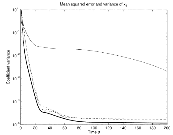
Fig. 1. Graphs of mean square error and estimation variance for EKF and UKF
In this figure, the thin line is the root mean square error for EKF (mean-squarred errors). Point graph (bold, at the very bottom) is an estimate of covariances (estimated covariances). Two other charts are for UKF. The EKF has less covariance estimates (it smooths out a little better), but the mean deviations are very high in his estimates. In the UKF, the covariances and the deviations are approximately at the same level. By the way, it seemed to me that there was some kind of mistake here. Dispersion is a square from the standard deviation. How can they be together? Here either I interpreted the terms incorrectly (I quoted them in parentheses above), or, nevertheless, the estimates of the covariances and the standard deviation are separate values.
UPD I also want to note that I myself have not yet fully understood how this method works, and whether I understood it correctly. I will try to implement it - it seems like an algorithm that is really easy to implement. I'll see how he shows himself how time will be.
In the meantime, your thoughts, suggestions, comments ... and THANKS FOR YOUR ATTENTION!

BIBLIOGRAPHY:

1. UKF at Wiki
2. A Discussion of Nonlinear Sigma Point Kalman Filter Orbit Determination
3. Julier, SJ; Uhlmann, JK (1997). “A new extension of the Kalman filter to nonlinear systems”. Int. Symp. Aerospace / Defense Sensing, Simul. and Controls 3. Retrieved 2008-05-03.
4. Fuzzy strong tracking unscented Kalman filter
5. Unscented Transform
6. M. Athans, RP Wishner, and A. Bertolini, “Suboptimal state
   estimation for continuous-time nonlinear systems from discrete
   noisy measurements, ”IEEE Trans. Automat. Contr., Vol. AC-13,
   pp. 504-518, Oct. 1968.