Kalman filter - is it difficult?

I recently read a post from Augmented Reality that mentions Kalman Filter in comparison to a simpler alpha beta filter. I have long been planning to compose something like a snippet for compiling a FC, and now I think it's about time. In the article I will tell you how in practice you can make an advanced FC without particularly troubling yourself with highly scientific reflections and deep theoretical research.

Basic concepts

1. The input-output equation is a differential equation (for example, composed by the Lagrange equations of the second kind), in which the left side of the equal sign contains terms depending on the output variable (the generalized coordinates of the system’s own motion), and on the right side the terms with input variable or free members. For simplicity, we can give the following example: for the pendulum, the left side of the "input-output" equation will be composed of terms with an angle of deviation of the load from the rest position, and on the right-hand side - the terms with gravity and other external forces. How I get such equations I will not describe - there is no need to complicate the publication of useless theoretical calculations. Below I will show that you can get by using convenient methods.
2. The transfer function (PF) is the ratio of the output to the input, or rather, the output variable to the input. According to the rule of proportion, after the removal of brain variables by brackets, the transfer function will be equal to the ratio of the left part, recorded in the operator form, to the right part.
3. Operator form of the record - the equation “input-output” is written in it after changing the form: s = d / dt and x (t) -> x (s). As a result, the equation of the form:
   a1 * x '' + a2 * x '+ a3 * x = b1 * u' + b2 * u,
   converted to the form:
   (a1 * s ^ 2 + a2 * s + a3) * x (s) = (b1 * s + b2) * u (s).
   In this case, the transfer function will be:
   W (s) = x (s) / u (s) = (b1 * s + b2) / (a1 * s ^ 2 + a2 * s + a3)

Task

As an application for the FC, we take the task of processing information of the sensor unit (see [1] ). We have four units of two-axis micromechanical accelerometers (MMA). Only 8 measuring channels, for each of which you can make a separate equation of the type "input-output". Here it should be noted that some of the manufacturers of sensors (for example, Analog Devices) provide an approximate linearized (this is important in our case) mathematical model. When working on a diploma, I received a model for MatLab from my colleagues. But even if the manufacturer clicks vigorously guards his secrets, the trouble is small. If we talk about accelerometers from AD, then their bandwidth for many practical tasks is large. For example, the ADXL203 band, if memory does not change, 10kHz. As an acoustic sensor, it does not roll (does not reach hundreds of kHz), and for civilian use on mobile objects (cars, yachts, scooters, bicycles, baby carriages) or in the gaming industry (it’s hardly possible for a person to wave with a frequency of 10 Hz ) such a band is excessive.
Thus, we ourselves can make the model of sensors we need. And in this way we kill two birds with one stone: we make up a simple linearized model and introduce noise filtering at the lowest level. About the simplicity of the model, it should be noted that when using an equation that accurately describes the dynamics of the sensor, we will be forced to compose the Kalman filter matrices from numbers whose orders are very different. In the “from the manufacturer” model for the accelerometers mentioned, the ratio of the maximum to the minimum coefficient is of the order of 1e + 10. This leads to severely low conditional calculations, i.e. a small error in setting the coefficient value can lead to a very large computational error. Narrowing the bandwidth embedded in the mathematical model, we essentially increase the stability of the calculations.
So how to make this very model? Yes, very simple. Using MatLab or Octave packages and specifying the bandwidth we need (LPF, HPF or bandpass filter), using a spear method or using plug-ins in packets, we synthesize the PF. It should be noted here that the MatLab package includes a visual means of synthesis of a discrete filter. In Octave, I haven’t found an analogue yet. In both packets, you can build frequency response and phase response graphs, which need to pay attention to the frequency (or frequencies) of the cutoff, as well as fluctuations in the frequency response graph in and out of the passband. In general, the shaman with the coefficients of the transfer function until the graphs of the frequency response and phase response does not satisfy us. For myself, I have already outlined another, more lazy simple way, namely, to use genetic algorithms for identification. It is only necessary to implement the reference samples "input - output" and organize the evolutionary process. But from a scientific point of view, the stated “methods” are invalid.

Mathematical model

And so for simplicity, we agree that there is an equation in operator form:

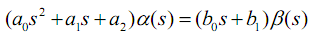
This is one of the most common second order dynamic equations. In this equation a2 - plays the role of the spring constant (the stiffness force is directly proportional to the distance of the position of the sensitive element from the rest position); 1 - damping coefficient (force proportional to the speed of movement; think of honey - it is easier to move the spoon in it slowly than quickly); a0 - characterizes inertia. In the coefficients to the right of the equal sign, a slightly different meaning is inserted. These coefficients characterize the effectiveness of exposure in different orders of derivatives. Here it is important to understand that the requirement of physical realizability limits the maximum order of the right derivative to the maximum order of the derivative of the left side.
Having obtained such an equation, we can begin the preparation for compiling the Kalman filter. To do this, we first need to convert the input-output equation to the state-space model. This is done using a transformation to the “Cauchy form”.
First you need to convert to the form of proportions and introduce a new (dummy) variable:

As a result, we obtain the system of equations:

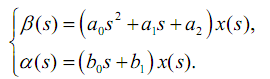
In this system, the first equation is the equation of the dynamic process, and the second is the equation of observation.
We give the first equation to the Cauchy form (to the system of first order differential equations) by replacing x1 = x:

For the convenience of recording replacements in this system, the inverse transformation was performed.
Laplace (transition from operator to differential form). As a result, we broke
original equation for two first order equations. The input variables x1 and x2 are called “state variables” or “phase coordinates”. The resulting system operates with "continuous" time. We made it according to the initial differential equations. But we need to build a difference algorithm (algorithm in discrete time) to calculate the value of phase coordinates in a recurrent way in a computer. Therefore, before using the Kalman filter, this system will need to be "sampled." But more about that later.
Now we need to make the observation equation for the entered phase coordinates. Taking into account
introduced substitutions and in differential form we get:

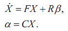
It remains to rewrite the resulting equations in vector-matrix form, pre-arranging the terms in accordance with the indices of the phase coordinates:

In this equation

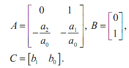
To discretize these equations, use the following expressions:

where I is the identity matrix, F and R are the desired discretized matrices of the state space model (difference equations), ts is the quantization period.
The quantization period is a key element in discretization. The smaller it is, the more accurate
repeats the discrete model behavior of the model with continuous time. Also, when
too large ts values ​​due to computational errors, the discrete model will become
unstable. If the object is not highly dynamic (for example, a low-pass filter with
bandwidth up to 10 Hz), then the quantization period can be chosen large enough. For
The quantization period mentioned in the low-pass filter can be selected with a large margin of 0.01 sec.
So, we have a discrete model of the form:

Now everything is ready for drawing up the FK model. We just have to build diagonally the F, R, and C matrixes for each measuring channel. For 8 measuring channels, for each of which a discrete own matrix F with dimensions of 2x2 is composed, we get our own Kalman filter matrix A (see the image at the beginning of the publication ) with sizes 16x16. We also deal with the column vector R: 2x1 * 8 channels = 16x8 - matrix B in the FK model. From the row vectors C, the matrix H is composed of a Kalman filter (8x16).
Done! Next you need to program it all. Personally, I prefer to use Ruby + NArray for this - it is a pleasure to prototype with this bundle, but this is my personal opinion ... as someone. Just keep in mind that you should not program these equations in the forehead - the resulting matrices are strongly sparse with zeros. If you think about it, then all matrix expressions can be divided into block operations. Here you need to optimize a lot of things at the implementation stage.

Conclusion

Sorry for some confusion in notation. Formulas were twitching from different works. I will try to briefly explain what is what in the equations of FC on the image at the beginning of the post.
The first thing that can be noticed is the matrices P, Q, R, K. These are, respectively, the covariance matrix of estimation errors (errors in solving the FK problem), the dynamic process noise and measurement noise covariations matrix, and the Kalman filter gain matrix. Vectors "x" and "z" are the phase vector of the PC (imitation of the phase vector of the sensor unit inside the FC model) and the vector of the output signals of the real sensors (in fact, it is a channel for receiving information from the outside in the FC). From the presented diagram it is easy to understand the principle of operation of FC.
It seems nothing complicated. However, in the work of FC there are a number of important nuances. So FC is designed as an algorithm that gives the smallest root-mean-square error if several conditions (hypotheses) are observed. First, the noises are white (uniform spectral characteristic) with a Gaussian distribution of random variables. But in practice, this hypothesis does not hold, because It is difficult to find a source of noise with such ideal parameters. In addition, the measuring systems themselves have finite bandwidths. In this case, the phase vector FC need to include more and variables for noise processes. An artificial approach is used: it is believed that we have a source of white noise, the signal from which passes through a filter. Thus, a model of two more dynamic objects is added to the FK model - filters that convert a pair of white noise processes into colored noise of the dynamic process and measurement noise.
The second hypothesis is the uncorrelated noise of different measuring channels. It is also rarely performed and again there are artificial methods to circumvent this limitation. All these methods lead to an increase in the dimensionality of the FK => increase the computational load.
The subtleties of the work of FC complicate the lives of botanists of scientists, but often for practical applications it is more important to reduce the dimension of FC rather than meet certain theoretical requirements. We are looking for an approximate solution by numerical methods, rather than an exact analytical solution with a clear theoretical justification. Although someone like ...

Bibliography

1. Non-orthogonal bees for small UAVs
2. habrahabr.ru/blogs/augmented_reality/118192
3. Brammer K., Ziffling G. Kalman-Bucy Filter. Per. with him. - M .: Science. the main
   editors of physical and mathematical literature. 1982
4. Sizikov V.S. Sustainable methods of processing measurement results. Tutorial.
   - SPb .: “SpecLit”, 1999. - 240 p.
5. Greg Welch, Gary Bishop. An Introduction to the Kalman Filter. TR 95-041, Department of
   Computer Science, University of North Carolina at Chapel Hill. April 5, 2004.