Counting objects in a binary image. Part 1

annotation

One, two, three, four, five. We will hide and seek we play. The article describes the algorithm for marking up (or counting) objects in a binary image and how the geometric characteristics of these objects are calculated (in the still unpublished part 2). Algorithms of this type are often used to recognize patterns on a binary preparation and show their computational efficiency.

At the end of the article, readers are offered an interesting problem, a competent solution of which exists and is necessary in the practical implementation of the algorithm. The source code is given, but unlike my previous posts, it is not made in MatLab but in an absolutely free, equally powerful SciLab environment.

Introduction

In practical applications designed for use in real time, pattern recognition is often performed in the following sequence:

Image acquisition (1) -> Adaptive binarization (2) -> A series of morphological operations (3) -> Object markup (4) -> Population of feature feature space (5).



Figure 1 - Simplified pattern of pattern recognition in the image. The scheme excludes the stages of separation of the space of signs and decision making



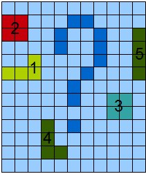
Figure 2 shows fragments of the image after binarization and a series of morphological operations (Fig. 2a) and the actual markup result (Fig. 2b).



Figure 2 - a) - binarized image, b) - image with marked-up objects.



In the article we will not only mark up objects, but also calculate geometrical characteristics such as area and perimeter. Their correlations can describe the compactness of an object and the Malinowski form factor, and in combination with more complex geometric features, elongation and contour features.

')

Scientifically, what we want to get is called selection of connected areas . There are many solutions to this problem - based on templates [1], some recursive implementations (for example, Listing 1 from [2]) and others.



void Labeling (BIT * img [], int * labels [])

{

int L = 1;

for ( int y = 0; y <H; ++ y)

for ( int x = 0; x <W; ++ x)

Fill (img, labels, x, y, L ++);

}

void Fill (BIT * img [], int * labels [], int x, int y, int L)

{

if ((labels [x] [y] == 0) & (img [x] [y] == 1))

{

labels [x] [y] = L;

if (x> 0)

Fill (img, labels, x - 1, y, L);

if (x <W - 1)

Fill (img, labels, x + 1, y, L);

if (y> 0)

Fill (img, labels, x, y - 1, L);

if (y <H - 1)

Fill (img, labels, x, y + 1, L);

}

}



* This source code was highlighted with Source Code Highlighter .

Listing 1 is a recursive implementation of the layout algorithm for connected domains.



All this does not suit us.

The region of pixels will be called connected if for each pixel from this region there is a neighbor from the same region. About the types of connectivity, I gave an illustration in this topic (Fig. 1,2). Our algorithm will be four connected, although it can also be altered for eight connected versions without much mental effort.

Single-pass, non-recursive markup algorithm

The idea of ​​this algorithm is based on the use of a corner - ABC-mask, which is shown in Figure 3.

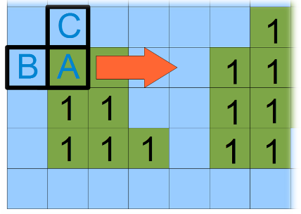
Figure 3 - ABC mask and the direction of sequential image scanning.



Pass through the image of this mask is carried out from left to right and top to bottom. It is believed that there are no objects abroad, therefore, if B or C falls there, this requires additional verification during scanning. Figure 4 shows 5 possible mask positions on the image.

Consider them.



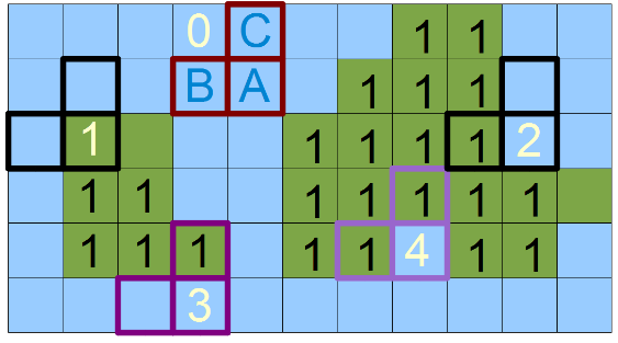
Figure 4 - Five possible positions of the ABC mask

1. Position number 0, when all three components of the mask are not marked - in this case, we simply skip the pixel.
2. Position number 1, when only element A is marked - in this case we are talking about creating a new object - a new number.
3. Position number 2 when element B is marked - in this case we mark the current pixel A with a label located in B.
4. Position number 3, when the element C is marked - in this case, we mark the current pixel A with a label located in C.
5. Position number 4, then we say that the labels (object numbers) B and C are connected - that is, they are equivalent and pixel A can be labeled either as B or as C. In some, the equivalence graph of such labels, followed by analysis, but in my opinion it is not necessary. We will do so - in the event that B is not equal to C, then we will renumber all already processed pixels marked as C in label B. But about this at the very end.

Closer to implementation.

At the beginning, we will create test data similar to those shown in Figure 2, namely the Image matrix consisting of zeros and ones.



Image = [0 0 0 0 0 0 0 1 0 0 0;

0 0 0 1 1 0 0 1 0 0 0;

0 0 0 1 1 0 0 1 1 0 0;

0 1 1 1 1 0 0 1 1 1 1;

0 1 1 1 1 0 0 0 0 0 0;

0 1 1 1 0 0 0 0 0 0 0;

0 0 0 0 0 0 0 0 0 0 0;

0 0 0 0 0 0 1 1 0 0;

0 0 0 0 0 0 1 1 1 0 0;

0 1 1 0 0 1 1 1 1 0 0;

0 1 1 0 0 1 1 1 1 1 1;

0 1 1 1 0 1 1 0 1 1 0;

0 0 0 0 0 0 0 0 0 0]

Matplot (Image * 255) // Let's look at our matrix like in the picture

[m, n] = size (Image); // Learn the horizontal and vertical dimensions of the matrix

km = 0; kn = 0; // They are still useful to us

cur = 1; // Variable for counting objects



* This source code was highlighted with Source Code Highlighter .

Listing 2 - initialization of the source data.



And then go through the image performing a series of simple and obvious checks. The ABC mask, which we pass through the picture, is illustrated in Figure 3. Possible combinations that are checked by this mask are shown in Figure 4.



// Cycle by image pixels

for i = 1: 1: m

for j = 1: 1: n

kn = j - 1;

if kn <= 0 then

kn = 1;

B = 0;

else

B = Image (i, kn); // See figure 3 in the article

end

km = i - 1;

if km <= 0 then

km = 1;

C = 0;

else

C = Image (km, j); // See figure 3 in the article

end

A = Image (i, j); // See figure 3 in the article

if A == 0 then // If the current pixel is empty, then we do nothing

elseif B == 0 & C == 0 then // If around our pixel is empty and it is not empty, then this is a reason to think about a new object.

cur = cur + 1;

Image (i, j) = cur;

elseif B ~ = 0 & C == 0 then

Image (i, j) = B;

elseif B == 0 & C ~ = 0 then

Image (i, j) = C;

elseif B ~ = 0 & C ~ = 0 then

if B == C then

Image (i, j) = B;

else

Image (i, j) = B;

Image (Image == C) = B;

end

end

end

end



* This source code was highlighted with Source Code Highlighter .

Listing 3 is a sequential scan of image pixels and layout of connected regions.



The result of the execution of this script will be the markup matrix:



Figure 5 - Result of the implementation of Listings 2 and 3 - objects are assigned unique numbers.



The disadvantage is that the numbers are not consistent, however, by and large this is absolutely not necessary, but it is corrected by additional modifications of the algorithm.



In conclusion of the first part of the article, the renumbering of labels can not be done at all, if the matrix of pointers to a special structure is used wisely. I propose to reflect on this to the reader. In the SciLab language, it will not be possible to implement a version with pointers, but in the last third part of the article I will do it using pseudo-code.



What will happen in the second part - it will be told about the empirical factors of the forms of objects, compactness and the Malinowski factor. We will look at a unique illustration on which I am currently working, on which a smooth change in the shape of an object is reflected by an increase or decrease in its factor-form.



Thanks to all who read, waiting for your feedback.

References and sources used

[1] Algorithms / Counting objects in the image link (apparently this article was once on Habré, but could not be found)

[2] Lecture: Analysis of the information contained in the image link to the ppt file