Graph visualization. Rib method
Sometimes it is useful to present the graph in graphical form, so that the structure is visible. There are dozens of examples where this might be useful: visualizing the hierarchy of classes and packages of the source code of a program, visualizing a social graph (the same Twitter or Facebook) or a citation graph (which publications are referenced), etc. But here's the bad luck: the number of edges in the graph is often so great that the graph drawn is simply impossible to disassemble. Take a look at this picture:
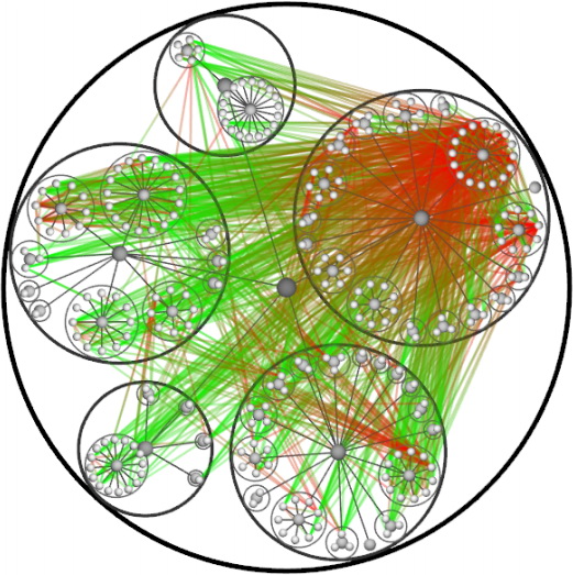
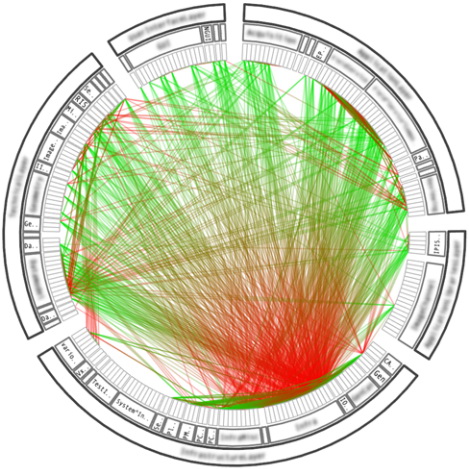
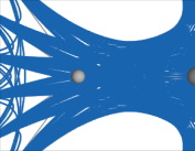
This is a dependency graph of a certain software system. It is a package tree (gray balls - packages, white - classes), on which are superimposed edges of the dependence of some classes on others. In order not to draw direction arrows, the edges are drawn as gradient lines, where green is the beginning and red is the end of the edge. As you can see, the graph is so visually overloaded that the architecture of the program can not be traced.
Under the cat description of the method that solves this problem.
')
The idea of the method is ingeniously simple - why not use the same principle as in cable networks? Many of us know which mess begins when the wires become too much. In order to prevent this mess, the wires are bundled together.
How to apply this idea to graphs and implement it algorithmically?
Consider an example of drawing one edge using an example. It is necessary to draw an edge from the vertex P 0 to the vertex P 4 :
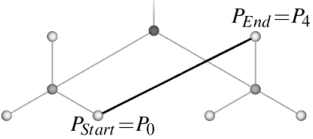
Find the path between these vertices:

Now draw a curve through the polygon formed by the points P 0 , P 1 , P 2 , P 3 , P 4 :
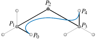
Actually, how to do it? The authors of this method analyzed that piecewise-specified cubic B-splines are best suited for visualization purposes. The problem of finding such B-splines is a classic one and has been solved by others long ago. In short, I’ll just say that a cubic B-spline is simply a set of third-order curves in two-dimensional space for which the stitching conditions of the first and second derivatives are met at the edges. If someone wants to implement this method, do not reinvent the wheel - at the end I laid out the working edge drawing code in C #.
In order to control the degree of connectivity of the edges, the parameter β is entered, which takes values from 0 to 1 (0 - the edges are not connected into a bundle and are independent straight lines, 1 - the edges are most connected with each other). Mathematically, it looks like this:

S (t) are spline points, S '(t) is the resulting curve, which is drawn on the screen as an edge.
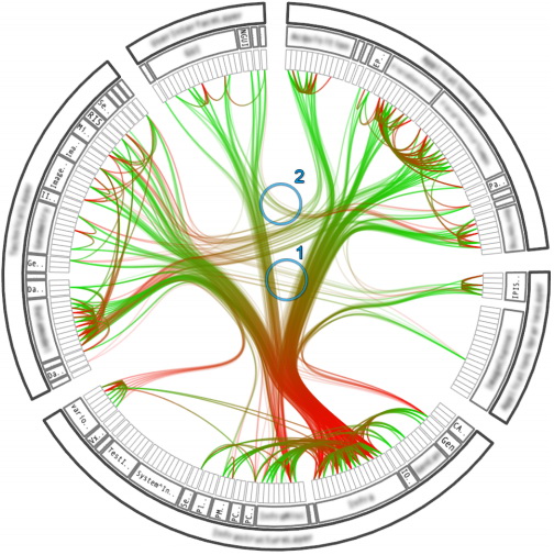
Well, here is the result of what all this math translates into:
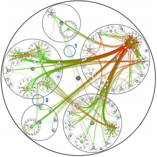
Here β = 0.85. Now the program's architecture is much clearer. One can see separate bundles of edges, dependencies between packages are visible.
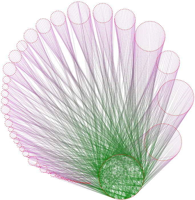
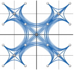
The same graph, only the radial method of visualizing the architecture is used (without applying the method, equivalent to β = 0):
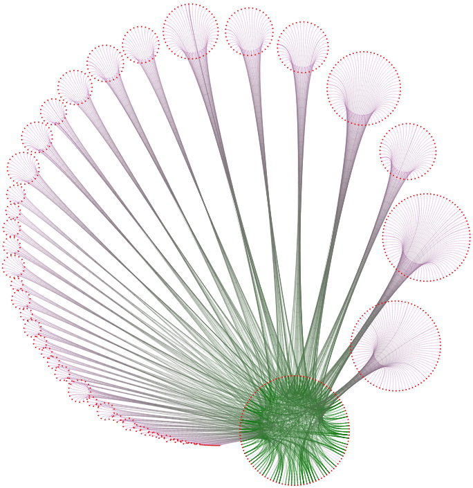
Using the method (β = 0.85):
As you can see, the method of linking the edges can be combined with various methods of drawing trees: this is its great advantage.
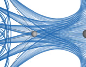
Graph citing publications. The green circle is 2008 publications that refer to publications from previous years (2007, 2006, etc.). Only links of 2008 publications are marked. Without applying the method, it looks like this:
Using the method (β = 0.99):
1. To avoid this:
You can use the alpha channel:
2. If we remove the LCA vertex from the control polygon (least common ancestor, the smallest common ancestor between the connected vertices), then the graph will look much better. Take a look at the difference:

In the second case, the LCA vertex is excluded from the vertex set, and the graph looks much more beautiful.
Below is the implementation of the System.Drawing.Graphics extension class, which can draw a cubic B-spline through a set of vertices.
The described method of linking edges and almost all the pictures are taken from the article “Hierarchical Edge Bundles:
Visualization of Adjacency Relations in Hierarchical Data. The author is Danny Holten.
This is a dependency graph of a certain software system. It is a package tree (gray balls - packages, white - classes), on which are superimposed edges of the dependence of some classes on others. In order not to draw direction arrows, the edges are drawn as gradient lines, where green is the beginning and red is the end of the edge. As you can see, the graph is so visually overloaded that the architecture of the program can not be traced.
Under the cat description of the method that solves this problem.
')
Method Description
The idea of the method is ingeniously simple - why not use the same principle as in cable networks? Many of us know which mess begins when the wires become too much. In order to prevent this mess, the wires are bundled together.
How to apply this idea to graphs and implement it algorithmically?
Consider an example of drawing one edge using an example. It is necessary to draw an edge from the vertex P 0 to the vertex P 4 :
Find the path between these vertices:
Now draw a curve through the polygon formed by the points P 0 , P 1 , P 2 , P 3 , P 4 :
Actually, how to do it? The authors of this method analyzed that piecewise-specified cubic B-splines are best suited for visualization purposes. The problem of finding such B-splines is a classic one and has been solved by others long ago. In short, I’ll just say that a cubic B-spline is simply a set of third-order curves in two-dimensional space for which the stitching conditions of the first and second derivatives are met at the edges. If someone wants to implement this method, do not reinvent the wheel - at the end I laid out the working edge drawing code in C #.
In order to control the degree of connectivity of the edges, the parameter β is entered, which takes values from 0 to 1 (0 - the edges are not connected into a bundle and are independent straight lines, 1 - the edges are most connected with each other). Mathematically, it looks like this:
S (t) are spline points, S '(t) is the resulting curve, which is drawn on the screen as an edge.
Well, here is the result of what all this math translates into:
Here β = 0.85. Now the program's architecture is much clearer. One can see separate bundles of edges, dependencies between packages are visible.
The same graph, only the radial method of visualizing the architecture is used (without applying the method, equivalent to β = 0):
Using the method (β = 0.85):
As you can see, the method of linking the edges can be combined with various methods of drawing trees: this is its great advantage.
Other examples
Graph citing publications. The green circle is 2008 publications that refer to publications from previous years (2007, 2006, etc.). Only links of 2008 publications are marked. Without applying the method, it looks like this:
Using the method (β = 0.99):
Remarks
1. To avoid this:
You can use the alpha channel:
2. If we remove the LCA vertex from the control polygon (least common ancestor, the smallest common ancestor between the connected vertices), then the graph will look much better. Take a look at the difference:
In the second case, the LCA vertex is excluded from the vertex set, and the graph looks much more beautiful.
C # implementation
Below is the implementation of the System.Drawing.Graphics extension class, which can draw a cubic B-spline through a set of vertices.
using System;
using System.Text;
using System.Drawing;

static class GraphicsExtension
{
private static void DrawCubicCurve( this Graphics graphics, Pen pen, float beta, float step, PointF start, PointF end, float a3, float a2, float a1, float a0, float b3, float b2, float b1, float b0)
{
float xPrev, yPrev;
float xNext, yNext;
bool stop = false ;

xPrev = beta * a0 + (1 - beta) * start.X;
yPrev = beta * b0 + (1 - beta) * start.Y;

for ( float t = step; ; t += step)
{
if (stop)
break ;

if (t >= 1)
{
stop = true ;
t = 1;
}

xNext = beta * (a3 * t * t * t + a2 * t * t + a1 * t + a0) + (1 - beta) * (start.X + (end.X - start.X) * t);
yNext = beta * (b3 * t * t * t + b2 * t * t + b1 * t + b0) + (1 - beta) * (start.Y + (end.Y - start.Y) * t);

graphics.DrawLine(pen, xPrev, yPrev, xNext, yNext);

xPrev = xNext;
yPrev = yNext;
}
}

/// <summary>
/// Draws a B-spline curve through a specified array of Point structures.
/// </summary>
/// <param name="pen">Pen for line drawing.</param>
/// <param name="points">Array of control points that define the spline.</param>
/// <param name="beta">Bundling strength, 0 <= beta <= 1.</param>
/// <param name="step">Step of drawing curve, defines the quality of drawing, 0 < step <= 1</param>
internal static void DrawBSpline( this Graphics graphics, Pen pen, PointF[] points, float beta, float step)
{
if (points == null )
throw new ArgumentNullException( "The point array must not be null." );

if (beta < 0 || beta > 1)
throw new ArgumentException( "The bundling strength must be >= 0 and <= 1." );

if (step <= 0 || step > 1)
throw new ArgumentException( "The step must be > 0 and <= 1." );

if (points.Length <= 1)
return ;

if (points.Length == 2)
{
graphics.DrawLine(pen, points[0], points[1]);
return ;
}

float a3, a2, a1, a0, b3, b2, b1, b0;
float deltaX = (points[points.Length - 1].X - points[0].X) / (points.Length - 1);
float deltaY = (points[points.Length - 1].Y - points[0].Y) / (points.Length - 1);
PointF start, end;

{
a0 = points[0].X;
b0 = points[0].Y;

a1 = points[1].X - points[0].X;
b1 = points[1].Y - points[0].Y;

a2 = 0;
b2 = 0;

a3 = (points[0].X - 2 * points[1].X + points[2].X) / 6;
b3 = (points[0].Y - 2 * points[1].Y + points[2].Y) / 6;

start = points[0];
end = new PointF
(
points[0].X + deltaX,
points[0].Y + deltaY
);

graphics.DrawCubicCurve(pen, beta, step, start, end, a3, a2, a1, a0, b3, b2, b1, b0);
}

for ( int i = 1; i < points.Length - 2; i++)
{
a0 = (points[i - 1].X + 4 * points[i].X + points[i + 1].X) / 6;
b0 = (points[i - 1].Y + 4 * points[i].Y + points[i + 1].Y) / 6;

a1 = (points[i + 1].X - points[i - 1].X) / 2;
b1 = (points[i + 1].Y - points[i - 1].Y) / 2;

a2 = (points[i - 1].X - 2 * points[i].X + points[i + 1].X) / 2;
b2 = (points[i - 1].Y - 2 * points[i].Y + points[i + 1].Y) / 2;

a3 = (-points[i - 1].X + 3 * points[i].X - 3 * points[i + 1].X + points[i + 2].X) / 6;
b3 = (-points[i - 1].Y + 3 * points[i].Y - 3 * points[i + 1].Y + points[i + 2].Y) / 6;

start = new PointF
(
points[0].X + deltaX * i,
points[0].Y + deltaY * i
);

end = new PointF
(
points[0].X + deltaX * (i + 1),
points[0].Y + deltaY * (i + 1)
);

graphics.DrawCubicCurve(pen, beta, step, start, end, a3, a2, a1, a0, b3, b2, b1, b0);
}

{
a0 = points[points.Length - 1].X;
b0 = points[points.Length - 1].Y;

a1 = points[points.Length - 2].X - points[points.Length - 1].X;
b1 = points[points.Length - 2].Y - points[points.Length - 1].Y;

a2 = 0;
b2 = 0;

a3 = (points[points.Length - 1].X - 2 * points[points.Length - 2].X + points[points.Length - 3].X) / 6;
b3 = (points[points.Length - 1].Y - 2 * points[points.Length - 2].Y + points[points.Length - 3].Y) / 6;

start = points[points.Length - 1];

end = new PointF
(
points[0].X + deltaX * (points.Length - 2),
points[0].Y + deltaY * (points.Length - 2)
);

graphics.DrawCubicCurve(pen, beta, step, start, end, a3, a2, a1, a0, b3, b2, b1, b0);
}
}
}

* This source code was highlighted with Source Code Highlighter .
Literature
The described method of linking edges and almost all the pictures are taken from the article “Hierarchical Edge Bundles:
Visualization of Adjacency Relations in Hierarchical Data. The author is Danny Holten.
Source: https://habr.com/ru/post/116758/
All Articles