Image Compression Algorithms
It is easy to calculate that an uncompressed full color image with a size of 2000 * 1000 pixels will be about 6 megabytes. If we talk about the images obtained from professional cameras or scanners of high resolution, then their size can be even larger. Despite the rapid growth in storage capacity, various image compression algorithms are still very relevant.
All existing algorithms can be divided into two large classes:
When we talk about lossless compression, we mean that there is an inverse of the compression algorithm that allows you to accurately restore the original image. For lossy compression algorithms, the inverse algorithm does not exist. There is an algorithm that restores the image does not necessarily exactly match the original one. Algorithms of compression and recovery are selected so as to achieve a high degree of compression and at the same time preserve the visual quality of the image.
All algorithms of the RLE series are based on a very simple idea: repeating groups of elements are replaced by a pair (number of repetitions, repeating element). Consider this algorithm on the example of a sequence of bits. In this sequence, groups of zeros and ones will alternate. And in groups there will often be more than one element. Then the sequence 11111 000000 11111111 00 will correspond to the next set of numbers 5 6 8 2. These numbers indicate the number of repetitions (counting starts from ones), but these numbers must also be encoded. We assume that the number of repetitions is in the range from 0 to 7 (i.e. we have enough 3 bits to encode the number of repetitions). Then the above sequence is encoded with the following sequence of numbers 5 6 7 0 1 2. It is easy to calculate that 21 bits are required for encoding the source sequence, and in the RLE-compressed form, this sequence takes 18 bits.
Although this algorithm is very simple, its effectiveness is relatively low. Moreover, in some cases, the use of this algorithm does not lead to a decrease, but to an increase in the length of the sequence. For example, consider the following sequence: 111 0000 11111111 00. The corresponding RL sequence looks like this: 3 4 7 0 1 2. The length of the original sequence is 17 bits, the length of the compressed sequence is 18 bits.
This algorithm is most effective for black and white images. It is also often used as one of the intermediate stages of compressing more complex algorithms.
The idea behind the vocabulary algorithms is that the chains of the elements of the original sequence are encoded. In this encoding, a special dictionary is used, which is obtained on the basis of the original sequence.
There is a whole family of dictionary algorithms, but we will look at the most common LZW algorithm, named after its developers Lepel, Ziv and Welch.
The dictionary in this algorithm is a table that is filled with coding chains as the algorithm works. When decoding compressed code, the dictionary is restored automatically, so there is no need to transfer the dictionary along with the compressed code.
The dictionary is initialized by all singleton chains, i.e. The first lines of the dictionary are the alphabet in which we perform the coding. During compression, the search for the longest chain is already recorded in the dictionary. Each time a chain is encountered that is not yet recorded in the dictionary, it is added there, and the compressed code corresponding to the chain already written in the dictionary is output. In theory, there are no restrictions on the size of the dictionary, but in practice it makes sense to limit this size, since with time the chains begin to occur, which are no longer found in the text. In addition, when increasing the size of the table in half, we must allocate an extra bit to store compressed codes. In order to prevent such situations, a special code is introduced, symbolizing the initialization of the table by all single-element chains.
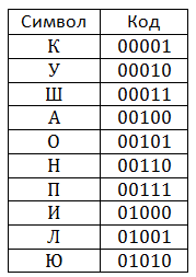
Consider an example of a compression algorithm. We will compress the string kukushkukkukushkukukupilkapushon. Suppose that the dictionary will hold 32 positions, which means that each code will occupy 5 bits. Initially the dictionary is filled as follows:
This table is, as well as on the side of the one who compresses the information, and on the side of the one who unpacks. We will now look at the compression process.
The table shows the process of filling the dictionary. It is easy to calculate that the resulting compressed code takes 105 bits, and the source text (provided that we spend 4 bits on coding one character) takes 116 bits.
In fact, the decoding process comes down to direct decoding of codes, while it is important that the table be initialized as well as during encoding. Now consider the decoding algorithm.

The line added to the dictionary on the i-th step can only be fully defined on i + 1. Obviously, the i-th line must end with the first character of i + 1 lines. So we just figured out how to restore the dictionary. Of some interest is the situation when a cScSc sequence is encoded, where c is one character and S is a string, and the word cS is already in the dictionary. At first glance, it may seem that the decoder cannot solve this situation, but in fact all lines of this type should always end with the same symbol on which they begin.
The algorithms of this series put the shortest compressed code as the most frequent elements of sequences. Those. sequences of the same length are encoded with compressed codes of different lengths. Moreover, the more frequent the sequence, the shorter the corresponding compressed code.
The Huffman algorithm allows you to build prefix codes. We can consider prefix codes as paths on a binary tree: passing from a node to its left son corresponds to 0 in the code, and to the right son to 1. If we mark the leaves of the tree with encoded characters, we get the representation of the prefix code as a binary tree.
We describe the algorithm for constructing a Huffman tree and obtaining Huffman codes.
Using this algorithm, we can get Huffman codes for a given alphabet, taking into account the frequency of occurrence of characters.
Arithmetic coding algorithms encode chains of elements in a fraction. This takes into account the frequency distribution of the elements. At the moment, the algorithms of arithmetic coding are protected by patents, so we consider only the basic idea.
Let our alphabet consist of N symbols a1, ..., aN, and the frequencies of their appearance p1, ..., pN, respectively. We divide the semi-interval [0; 1) into N disjoint semi-intervals. Each half-interval corresponds to the elements ai, and the length of the half-interval is proportional to the frequency pi.
The coding fraction is constructed as follows: a system of nested intervals is constructed so that each subsequent half-interval occupies the previous position corresponding to the position of the element in the original partition. After all the intervals are nested into each other, you can take any number from the resulting half-interval. Writing this number in binary code will be a compressed code.
Decoding - decoding fractions by a known probability distribution. Obviously, for decoding, it is necessary to store a table of frequencies.
Arithmetic coding is extremely efficient. Codes obtained with its help, approaching the theoretical limit. This suggests that as patents expire, arithmetic coding will become more and more popular.
Despite the many highly efficient lossless compression algorithms, it becomes obvious that these algorithms do not provide (and cannot provide) a sufficient degree of compression.
Lossy compression (applied to images) is based on the characteristics of human vision. We consider the basic ideas underlying the JPEG image compression algorithm.
JPEG is currently one of the most common ways to compress lossy images. We describe the basic steps underlying this algorithm. We assume that an image with a color depth of 24 bits per pixel arrives at the input of the compression algorithm (the image is presented in the RGB color model).
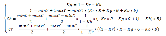
In the color model YCbCr, we present the image as a luminance component (Y) and two color difference components (Cb, Cr). The human eye is more susceptible to brightness, not to color, so the JPEG algorithm makes minimal changes to the luminance component (Y), and significant changes can be made to the color difference components. Translation is carried out according to the following formula:
The choice of Kr and Kb depends on the equipment. Usually, Kb = 0.114; Kr = 0.299. Recently, Kb = 0.0722; Kr = 0.2126 is also used, which better reflects the characteristics of modern display devices.
After translation into the YCbCr color space, sampling is performed. One of three sampling methods is possible:
four
When using the second or third method, we get rid of 1/3 or 1/2 of the information, respectively. Obviously, the more information we lose, the more distortions will be in the final image.
The image is divided into components of 8 * 8 pixels, DCT will be applied to each component. This leads to compaction of energy in the code. Transformations are applied to components independently.
A person is practically incapable of noticing changes in high-frequency components, therefore the coefficients responsible for high frequencies can be stored with less accuracy. For this purpose, component-wise multiplication (and rounding) of the matrices obtained as a result of DCT by the quantization matrix is used. At this stage, you can also adjust the degree of compression (the closer to zero the components of the quantization matrix, the smaller will be the range of the final matrix).
Zigzag-traversal of the matrix is a special direction of traversal, presented in the figure:

At the same time, for the majority of real images, nonzero coefficients will appear at the beginning, and zeros will go towards the end.
A special type of RLE encoding is used: pairs of numbers are output, the first number in the pair encodes the number of zeros, and the second the value after the sequence of zeros. Those. the code for the sequence 0 0 15 42 0 0 0 44 is as follows (2; 15) (0; 42) (3; 44).
The Huffman algorithm described above is used. Encoding uses a predefined table.
The decoding algorithm consists in reversing the executed transformations.
The advantages of the algorithm include a high degree of compression (5 or more times), relatively low complexity (taking into account special processor instructions), patent purity. The disadvantage is artifacts visible to the human eye.
Fractal compression is a relatively new area. A fractal is a complex geometric shape with a property of self-similarity. Algorithms of fractal compression are now actively developing, but the ideas underlying them can be described by the following sequence of actions.
Compression process:
Stages of image recovery:
The accuracy of the resulting image depends on the accuracy of the affine transformation.
The complexity of the fractal compression algorithms is that it uses integer arithmetic and special rather complex methods that reduce rounding errors.
A distinctive feature of fractal compression is its pronounced asymmetry. The compression and recovery algorithms differ significantly (compression requires much more computation).
All existing algorithms can be divided into two large classes:
- Lossless compression algorithms;
- Lossy compression algorithms.
When we talk about lossless compression, we mean that there is an inverse of the compression algorithm that allows you to accurately restore the original image. For lossy compression algorithms, the inverse algorithm does not exist. There is an algorithm that restores the image does not necessarily exactly match the original one. Algorithms of compression and recovery are selected so as to achieve a high degree of compression and at the same time preserve the visual quality of the image.
Lossless compression algorithms
RLE algorithm
All algorithms of the RLE series are based on a very simple idea: repeating groups of elements are replaced by a pair (number of repetitions, repeating element). Consider this algorithm on the example of a sequence of bits. In this sequence, groups of zeros and ones will alternate. And in groups there will often be more than one element. Then the sequence 11111 000000 11111111 00 will correspond to the next set of numbers 5 6 8 2. These numbers indicate the number of repetitions (counting starts from ones), but these numbers must also be encoded. We assume that the number of repetitions is in the range from 0 to 7 (i.e. we have enough 3 bits to encode the number of repetitions). Then the above sequence is encoded with the following sequence of numbers 5 6 7 0 1 2. It is easy to calculate that 21 bits are required for encoding the source sequence, and in the RLE-compressed form, this sequence takes 18 bits.
Although this algorithm is very simple, its effectiveness is relatively low. Moreover, in some cases, the use of this algorithm does not lead to a decrease, but to an increase in the length of the sequence. For example, consider the following sequence: 111 0000 11111111 00. The corresponding RL sequence looks like this: 3 4 7 0 1 2. The length of the original sequence is 17 bits, the length of the compressed sequence is 18 bits.
This algorithm is most effective for black and white images. It is also often used as one of the intermediate stages of compressing more complex algorithms.
Dictionary algorithms
The idea behind the vocabulary algorithms is that the chains of the elements of the original sequence are encoded. In this encoding, a special dictionary is used, which is obtained on the basis of the original sequence.
There is a whole family of dictionary algorithms, but we will look at the most common LZW algorithm, named after its developers Lepel, Ziv and Welch.
The dictionary in this algorithm is a table that is filled with coding chains as the algorithm works. When decoding compressed code, the dictionary is restored automatically, so there is no need to transfer the dictionary along with the compressed code.
The dictionary is initialized by all singleton chains, i.e. The first lines of the dictionary are the alphabet in which we perform the coding. During compression, the search for the longest chain is already recorded in the dictionary. Each time a chain is encountered that is not yet recorded in the dictionary, it is added there, and the compressed code corresponding to the chain already written in the dictionary is output. In theory, there are no restrictions on the size of the dictionary, but in practice it makes sense to limit this size, since with time the chains begin to occur, which are no longer found in the text. In addition, when increasing the size of the table in half, we must allocate an extra bit to store compressed codes. In order to prevent such situations, a special code is introduced, symbolizing the initialization of the table by all single-element chains.
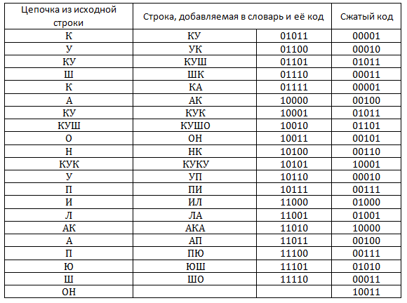
Consider an example of a compression algorithm. We will compress the string kukushkukkukushkukukupilkapushon. Suppose that the dictionary will hold 32 positions, which means that each code will occupy 5 bits. Initially the dictionary is filled as follows:
This table is, as well as on the side of the one who compresses the information, and on the side of the one who unpacks. We will now look at the compression process.
The table shows the process of filling the dictionary. It is easy to calculate that the resulting compressed code takes 105 bits, and the source text (provided that we spend 4 bits on coding one character) takes 116 bits.
In fact, the decoding process comes down to direct decoding of codes, while it is important that the table be initialized as well as during encoding. Now consider the decoding algorithm.
The line added to the dictionary on the i-th step can only be fully defined on i + 1. Obviously, the i-th line must end with the first character of i + 1 lines. So we just figured out how to restore the dictionary. Of some interest is the situation when a cScSc sequence is encoded, where c is one character and S is a string, and the word cS is already in the dictionary. At first glance, it may seem that the decoder cannot solve this situation, but in fact all lines of this type should always end with the same symbol on which they begin.
Algorithms of statistical coding
The algorithms of this series put the shortest compressed code as the most frequent elements of sequences. Those. sequences of the same length are encoded with compressed codes of different lengths. Moreover, the more frequent the sequence, the shorter the corresponding compressed code.
Huffman Algorithm
The Huffman algorithm allows you to build prefix codes. We can consider prefix codes as paths on a binary tree: passing from a node to its left son corresponds to 0 in the code, and to the right son to 1. If we mark the leaves of the tree with encoded characters, we get the representation of the prefix code as a binary tree.
We describe the algorithm for constructing a Huffman tree and obtaining Huffman codes.
- The characters in the input alphabet form a list of free nodes. Each sheet has a weight that is equal to the frequency of the symbol
- Two loose tree nodes with the smallest weights are selected.
- Their parent is created with a weight equal to their total weight.
- The parent is added to the list of free nodes, and his two children are removed from this list.
- One arc going out of the parent is assigned bit 1, the other is bit 0
- Steps, starting with the second, are repeated until only one free node remains in the list of free nodes. It will be considered the root of the tree.
Using this algorithm, we can get Huffman codes for a given alphabet, taking into account the frequency of occurrence of characters.
Arithmetic coding
Arithmetic coding algorithms encode chains of elements in a fraction. This takes into account the frequency distribution of the elements. At the moment, the algorithms of arithmetic coding are protected by patents, so we consider only the basic idea.
Let our alphabet consist of N symbols a1, ..., aN, and the frequencies of their appearance p1, ..., pN, respectively. We divide the semi-interval [0; 1) into N disjoint semi-intervals. Each half-interval corresponds to the elements ai, and the length of the half-interval is proportional to the frequency pi.
The coding fraction is constructed as follows: a system of nested intervals is constructed so that each subsequent half-interval occupies the previous position corresponding to the position of the element in the original partition. After all the intervals are nested into each other, you can take any number from the resulting half-interval. Writing this number in binary code will be a compressed code.
Decoding - decoding fractions by a known probability distribution. Obviously, for decoding, it is necessary to store a table of frequencies.
Arithmetic coding is extremely efficient. Codes obtained with its help, approaching the theoretical limit. This suggests that as patents expire, arithmetic coding will become more and more popular.
Lossy Compression Algorithms
Despite the many highly efficient lossless compression algorithms, it becomes obvious that these algorithms do not provide (and cannot provide) a sufficient degree of compression.
Lossy compression (applied to images) is based on the characteristics of human vision. We consider the basic ideas underlying the JPEG image compression algorithm.
JPEG compression algorithm
JPEG is currently one of the most common ways to compress lossy images. We describe the basic steps underlying this algorithm. We assume that an image with a color depth of 24 bits per pixel arrives at the input of the compression algorithm (the image is presented in the RGB color model).
Conversion to YCbCr color space
In the color model YCbCr, we present the image as a luminance component (Y) and two color difference components (Cb, Cr). The human eye is more susceptible to brightness, not to color, so the JPEG algorithm makes minimal changes to the luminance component (Y), and significant changes can be made to the color difference components. Translation is carried out according to the following formula:
The choice of Kr and Kb depends on the equipment. Usually, Kb = 0.114; Kr = 0.299. Recently, Kb = 0.0722; Kr = 0.2126 is also used, which better reflects the characteristics of modern display devices.
Downsampling the chroma component
After translation into the YCbCr color space, sampling is performed. One of three sampling methods is possible:
four
- : 4: 4 - no subsampling;
- 4: 2: 2 - components of chromaticity vary through one horizontally;
- 4: 2: 0 - the chromaticity components change through a single line horizontally, while vertically they change through a line.
When using the second or third method, we get rid of 1/3 or 1/2 of the information, respectively. Obviously, the more information we lose, the more distortions will be in the final image.
Discrete cosine transform
The image is divided into components of 8 * 8 pixels, DCT will be applied to each component. This leads to compaction of energy in the code. Transformations are applied to components independently.
Quantization
A person is practically incapable of noticing changes in high-frequency components, therefore the coefficients responsible for high frequencies can be stored with less accuracy. For this purpose, component-wise multiplication (and rounding) of the matrices obtained as a result of DCT by the quantization matrix is used. At this stage, you can also adjust the degree of compression (the closer to zero the components of the quantization matrix, the smaller will be the range of the final matrix).
Zigzag-traversal of matrices
Zigzag-traversal of the matrix is a special direction of traversal, presented in the figure:
At the same time, for the majority of real images, nonzero coefficients will appear at the beginning, and zeros will go towards the end.
RLE coding
A special type of RLE encoding is used: pairs of numbers are output, the first number in the pair encodes the number of zeros, and the second the value after the sequence of zeros. Those. the code for the sequence 0 0 15 42 0 0 0 44 is as follows (2; 15) (0; 42) (3; 44).
Huffman coding
The Huffman algorithm described above is used. Encoding uses a predefined table.
The decoding algorithm consists in reversing the executed transformations.
The advantages of the algorithm include a high degree of compression (5 or more times), relatively low complexity (taking into account special processor instructions), patent purity. The disadvantage is artifacts visible to the human eye.
Fractal compression
Fractal compression is a relatively new area. A fractal is a complex geometric shape with a property of self-similarity. Algorithms of fractal compression are now actively developing, but the ideas underlying them can be described by the following sequence of actions.
Compression process:
- Splitting an image into non-overlapping areas (domains). The domain set must cover the entire image.
- Selection of rank areas. Ranked areas may overlap and not cover the entire image.
- Fractal transformation: for each domain, such a ranking area is selected that, after affine transformation, most closely approximates the domain.
- Compress and save affine transform parameters. The file contains information about the location of domains and rank areas, as well as compressed coefficients of affine transformations.
Stages of image recovery:
- Creating two images of the same size A and B. The size and content of the areas do not matter.
- Image B is divided into domains in the same way as in the first stage of the compression process. For each domain of the domain B, the corresponding affine transformation of the ranking regions of the image A, described by coefficients from the compressed file, is carried out. The result is placed in area B. After the conversion, a completely new image is obtained.
- Converting data from area B to area A. This step repeats step 3, only images A and B are swapped.
- Steps 3 and 4 are repeated until images A and B become indistinguishable.
The accuracy of the resulting image depends on the accuracy of the affine transformation.
The complexity of the fractal compression algorithms is that it uses integer arithmetic and special rather complex methods that reduce rounding errors.
A distinctive feature of fractal compression is its pronounced asymmetry. The compression and recovery algorithms differ significantly (compression requires much more computation).
')
Source: https://habr.com/ru/post/116697/
All Articles