Classification and regression using decision trees

Introduction

This article provides an overview of decision trees (Decision trees) and three main algorithms that use these trees to build classification and regression models. In turn, it will be shown how the decision-making trees, initially focused on classification, are used for regression.

Decision Trees

A decision tree is a tree, in the leaves of which there are values ​​of the objective function, and in the remaining nodes there are transition conditions (for example, “FLOOR is MALE”) that determine which of the edges to go. If, for a given observation, the condition is true, then a transition is made along the left edge, if false, on the right.

Classification

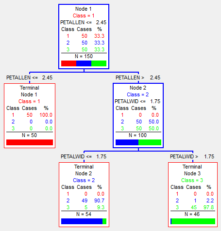
The image above shows an iris classification tree. The classification goes into three classes (marked on the image - red, blue and green), and passes by the parameters: the length / thickness of the sepal (SepalLen, SepalWid) and the length / thickness of the petal (PetalLen, PetalWid). As you can see, in each node it is worth belonging to a class (depending on which elements fall more into this node), the number of observations made there N, as well as the number of each class. Also not in leaf vertices there is a condition of transition - to one of the children. Accordingly, the sample is divided by these conditions. As a result, this tree almost perfectly (6 out of 150 incorrectly) classified the initial data (namely, the initial ones - the ones on which it was trained).
')

Regression

If the classification in sheets are the resulting classes, with regression, there is some value of the objective function.


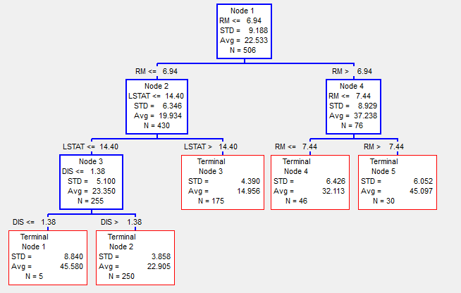
In the above image, a regression tree is used to determine the price of land in the city of Boston in 1978, depending on the parameters RM - the number of rooms, LSTAT - the percentage of poor people and several other parameters (see [4] for more details). Accordingly, here at each node we see the mean value (Avg) and standard deviation (STD) of the values ​​of the objective function of observations that fell at this vertex. The total number of observations hit the node N. The result of the regression will be the value of the average (Avg), which node will get the observation.
Thus, initially the classification tree can work for regression. However, with this approach, a large tree size is usually required than with a classification in order to achieve good regression results.

Basic methods

Below are a few basic methods that use decision trees. Their brief description, pros and cons.

CART

CART (Eng. Classification and regression trees - Classification and regression trees) was the first method invented in 1983 by four well-known scientists in the field of data analysis: Leo Breiman, Jerome Friedman, Richard Olshen and Stone [1].
The essence of this algorithm is the usual construction of a decision tree, no more and no less.
At the first iteration, we build all possible (in a discrete sense) hyperplanes that would divide our space into two. For each such partition of space, the number of observations in each of the subspaces of different classes is considered. As a result, such a partition is chosen that maximally distinguishes the observation of one of the classes in one of the subspaces. Accordingly, this partition will be our decision-making root, and the sheets in this iteration will be two partitions.
At the next iterations, we take one worst (in the sense of the ratio of the number of observations of different classes) sheet and carry out the same operation to split it. As a result, this sheet becomes a node with some sort of splitting, and two sheets.
We continue to do this until we reach the limit on the number of nodes, or the total error ceases to improve from one iteration to another (the number of incorrectly classified observations by the whole tree). However, the resulting tree will be “retrained” (will be fitted to the training sample) and, accordingly, will not give normal results on other data. In order to avoid “retraining”, test samples are used (or cross-validation) and, accordingly, a reverse analysis is performed (the so-called pruning), when the tree is reduced depending on the result on the test sample.
A relatively simple algorithm that results in a single decision tree. Due to this, it is convenient for primary data analysis, for example, to check for connections between variables and another.
Quick model building
Easy to interpret (because of the simplicity of the model, you can easily display the tree and follow all the nodes of the tree)
Often converges on a local solution (for example, at the first step a hyperplane was chosen that maximally divides the space at this step, but at the same time it does not lead to an optimal solution)

RandomForest

Random forest (Random Forest) - a method invented after CART by one of the four - Leo Breiman in collaboration with Adele Cutler [2], which is based on the use of the committee (ensemble) decision trees.
The essence of the algorithm is that at each iteration a random selection of variables is made, after which, at this new sample, the decision tree is built. This is “bagging” - a sample of a random two-thirds of the observations for training, and the remaining third is used to evaluate the result. Such an operation is done hundreds or thousands of times. The resulting model will be the result of “voting” a set of trees obtained in the simulation.
High quality results, especially for data with a large number of variables and a small number of observations.
The ability to parallelize
No test sample required.
Each of the trees is huge, as a result, the model is huge
Long model building, to achieve good results.
Complex interpretation of the model (Hundreds or thousands of large trees are difficult to interpret)

Stochastic Gradient Boosting

Stochastic Gradient Boosting (Stochastic Gradient Addition) is a data analysis method presented by Jerome Friedman [3] in 1999, which represents a solution to a regression problem (to which classification can be reduced) by building a committee (ensemble) of “weak” predictive decision trees.
At the first iteration, a decision tree is bounded by the number of nodes. After that, the difference between what the predicted tree multiplied by learnrate (the coefficient of “weakness” of each tree) and the desired variable at this step is calculated.
Yi + 1 = Yi-Yi * learnrate
And already on this difference the following iteration is under construction. This continues until the result ceases to improve. Those. at each step we try to correct the errors of the previous tree. However, it is better to use verification data here (not participating in the simulation), since retraining is possible on the training data.
High quality results, especially for data with a large number of observations and a small number of variables.
Comparatively (with the previous method), the small size of the model, since each tree is limited to given sizes.
Comparatively (with the previous method) fast time building an optimal model
Test sample required (or cross-validation)
Inability to parallelize well
Relatively weak tolerance for erroneous data and retraining
Difficult interpretation of the model (As in the Random forest)

Conclusion

As we have seen, each method has its pros and cons, and accordingly, depending on the task and the initial data, you can use one of the three methods to solve and get the desired result. However, CART is more used in universities for teaching and research, when some clear descriptive basis is needed for a solution (as in the above example of analyzing the price of land in Boston). And to solve industrial problems usually use one of his descendants - Random Forest or TreeNet.
These methods can be found in many modern packages for data analysis:

• Salford Predictive Modeling Suite
• Spss
• SAS
• Data analysis packages for project R

Bibliography

1. “Classification and Regression Trees”. Breiman L., Friedman JH, Olshen R. A, Stone CJ
2. “Random Forests”. Breiman L.
3. “Stochastic Gradient Boosting”. Friedman jh
4. http://www.cs.toronto.edu/~delve/data/boston/bostonDetail.html