Image fill algorithms, popular with video
annotation

Filling images is often a practical task, the essence of which is to fill a certain area of an image, bounded by a contour defined by color. And it would seem simple, but often slow and crooked. This article describes the well-known stack-based fill algorithms and provides an implementation in MatLab pseudo-code. I tried to fill such a boring topic with interesting video clips, and described the process of obtaining them, again using MatLab. In this article we will fill in Carlson who lives on the roof, as I did not find the habro-type for this purpose in normal resolution. As well as a few lines of code on how to read and work with pictures in MatLab.
Preliminary information and background
In a simple way, we introduce the relation of connectivity or neighborhood on an ordered set of pairs of coordinates. We will distinguish cases when a point has four neighbors (Fig.1a) and a case when a point has eight neighbors (Fig.1b).
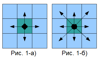
Why do it and what to choose is shown in Figure 2.
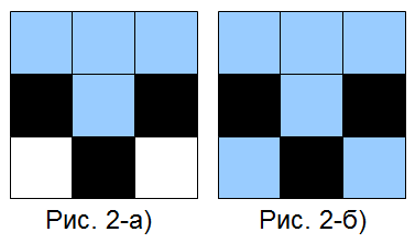
In Figure 2, the squares depict conventional pixels of a digital image, with black pixels describing the boundary between two areas — the upper and the lower. We will fill the top white area with blue paint. If we enter only 4 neighbors for a point, the blue paint will not pass through the black border (Fig.2b) and the lower area will remain white, and if we use eight neighbors, then the black border and not the border at all, but the sieve through which and paint is spilled into the lower area.
What kind of connectivity to choose? On the plane, the choice is small - either 4 or 8 neighbors and the choice depends on the formulation of the original problem, but in a multidimensional space it is more and more difficult, even impossible to imagine, and in the article we will consider only the flat case. In this case, we consider the case of four neighbors, which in a simple way extends to the case of eight.
')
 Everyone noticed that the picture of Carlson, painted according to my taste and presentation in Paint, in the annotation of the article, is somehow crooked, is there a black outline on the border - a colored area - are there white and gray, eye-catching points? This happened for the reason that our Carlson is not at all in binary color but in grayscale. First of all, we remove this glaring flaw and binarize the picture, while we only need to work with one channel - let it be the first - red.
So:
% //
source_image = imread( 'karlson.bmp' );
% //
gray_image = source_image(:,:,1);
% // 0.5
bim=double(im2bw(gray_image, 0.5));
% //
imagesc(bim);

* This source code was highlighted with Source Code Highlighter .
% //
source_image = imread( 'karlson.bmp' );
% //
gray_image = source_image(:,:,1);
% // 0.5
bim=double(im2bw(gray_image, 0.5));
% //
imagesc(bim);
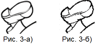
* This source code was highlighted with Source Code Highlighter .Figure 3 shows the leg of our mischief in its original form (Fig. 3a) and after binarization (Fig. 3b), as we see, the contour has become expectedly thinner and now consists only of black dots, while some of the boundaries have disappeared.
Next, we will look at two fill algorithms, but we will not program them recursively (so as not to dilute the extra holivars and avoid overflows), but expand the recursion to the stack.
We define the terminology:
- The starting point is the pixel in which the user pressed like a Point with a can of paint
- Old color - color of the area to be filled
- New color - the color of the area after the fill.
Simple and slow fill algorithm
The edges of the image will also be considered the border of the image.
The essence of the algorithm is simple: at the current point we check: if the old color is replace it with a new one, if it is new, then we do nothing. Then we perform the same operation for four neighbors whose color is equal to the old color.
Let me once steal the source code , with a recursive implementation, just to show the point:
//Recursive 4-way floodfill, crashes if recursion stack is full
void floodFill4( int x, int y, int newColor, int oldColor)
{
if (x >= 0 && x < w && y >= 0 && y < h && screenBuffer[x][y] == oldColor && screenBuffer[x][y] != newColor)
{
screenBuffer[x][y] = newColor; //set color before starting recursion

floodFill4(x + 1, y, newColor, oldColor);
floodFill4(x - 1, y, newColor, oldColor);
floodFill4(x, y + 1, newColor, oldColor);
floodFill4(x, y - 1, newColor, oldColor);
}
}
* This source code was highlighted with Source Code Highlighter .
//Recursive 4-way floodfill, crashes if recursion stack is full
void floodFill4( int x, int y, int newColor, int oldColor)
{
if (x >= 0 && x < w && y >= 0 && y < h && screenBuffer[x][y] == oldColor && screenBuffer[x][y] != newColor)
{
screenBuffer[x][y] = newColor; //set color before starting recursion
floodFill4(x + 1, y, newColor, oldColor);
floodFill4(x - 1, y, newColor, oldColor);
floodFill4(x, y + 1, newColor, oldColor);
floodFill4(x, y - 1, newColor, oldColor);
}
}
* This source code was highlighted with Source Code Highlighter .What will it look like on Matlab with a stack imitation? That's how:
%
source_image = imread( 'karlson.bmp' );
%
gray_image = source_image(:,:,1);
% 0.5
bim= double (im2bw(gray_image, 0.5));
%
imagesc(bim);

newColor = 0.5; oldColor = 1;
point.x = 48; point.y = 234;
stack = [point];
[wh] = size(bim);
stack_size = [];
mov = avifile( 'karlson_fill2.avi' , 'fps' ,50);
figure;
while (length(stack) ~=0)
point = stack(1);
stack(1) = []; %
bim(point.x,point.y) = newColor; %

if (point.x+1 <= w && bim(point.x+1,point.y) == oldColor)
newpoint.x = point.x+1;
newpoint.y = point.y;
stack = [stack newpoint];
end;
if (point.x-1 > 0 && bim(point.x-1,point.y) == oldColor)
newpoint.x = point.x-1;
newpoint.y = point.y;
stack = [stack newpoint];
end;
if (point.y+1 <= h && bim(point.x,point.y+1) == oldColor)
newpoint.x = point.x;
newpoint.y = point.y+1;
stack = [stack newpoint];
end;
if (point.y-1 > 0 && bim(point.x,point.y-1) == oldColor)
newpoint.x = point.x;
newpoint.y = point.y-1;
stack = [stack newpoint];
end;
stack_size = [stack_size length(stack)];
imagesc(bim); colormap gray; axis image;
F = getframe(gca); mov = addframe(mov,F);
end;
mov = close(mov);
figure; imagesc(bim);
figure; plot(stack_size);

* This source code was highlighted with Source Code Highlighter .
%
source_image = imread( 'karlson.bmp' );
%
gray_image = source_image(:,:,1);
% 0.5
bim= double (im2bw(gray_image, 0.5));
%
imagesc(bim);
newColor = 0.5; oldColor = 1;
point.x = 48; point.y = 234;
stack = [point];
[wh] = size(bim);
stack_size = [];
mov = avifile( 'karlson_fill2.avi' , 'fps' ,50);
figure;
while (length(stack) ~=0)
point = stack(1);
stack(1) = []; %
bim(point.x,point.y) = newColor; %
if (point.x+1 <= w && bim(point.x+1,point.y) == oldColor)
newpoint.x = point.x+1;
newpoint.y = point.y;
stack = [stack newpoint];
end;
if (point.x-1 > 0 && bim(point.x-1,point.y) == oldColor)
newpoint.x = point.x-1;
newpoint.y = point.y;
stack = [stack newpoint];
end;
if (point.y+1 <= h && bim(point.x,point.y+1) == oldColor)
newpoint.x = point.x;
newpoint.y = point.y+1;
stack = [stack newpoint];
end;
if (point.y-1 > 0 && bim(point.x,point.y-1) == oldColor)
newpoint.x = point.x;
newpoint.y = point.y-1;
stack = [stack newpoint];
end;
stack_size = [stack_size length(stack)];
imagesc(bim); colormap gray; axis image;
F = getframe(gca); mov = addframe(mov,F);
end;
mov = close(mov);
figure; imagesc(bim);
figure; plot(stack_size);
* This source code was highlighted with Source Code Highlighter .You can go to drink tea, while the brow of our dandy is painted gray. At the same time, the proposed code will also draw us a chart of the stack fullness at each iteration and we will discuss it. And as a nice bonus code - the output also includes a video clip illustrating the filling. Why I chose such a small detail as an eyebrow - because it is not possible to fill in something else, such as a belly, taking into account the features of the Matlab language, in a finite time.
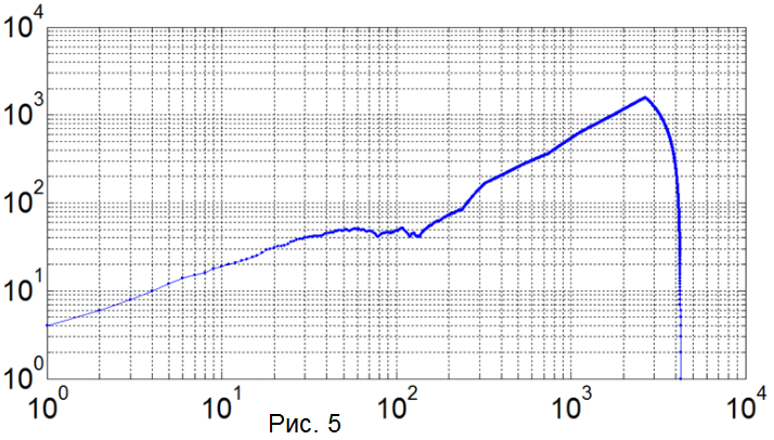
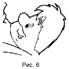 Actually, here are our results: The graph of the stack is shown in logarithmic coordinates in Figure 5.
And the head with a colored eyebrow is depicted in Figure 6. A video illustrating the process of filling the area is proposed for viewing below. Everything tells us that the algorithm works extremely slowly, look at Figure 5 (on the X axis - the iteration number, on the Y axis - the number of still raw points) how slowly the stack is emptied (consider the logarithmic coordinates), but the thing is There are too many unnecessary check points. Those points that were filled at the previous stage are still checked at the following. Of course this is no good. Next, we will eliminate this injustice! Video file - 50 frames per second.
Fill Algorithm - Fast, Lines
The essence of the recursive algorithm:
We start to fill the current line from one edge to another.
First up from the starting point and then down.
We return to the starting point. We look - if to the left of the starting point the old color and there is no border, then we fill the new line.
We return to the starting point. We look - if to the right of the starting point the old color and there is no border, then we fill the new line.
Algorithm code:
clear all;
%
source_image = imread( 'karlson.bmp' );
%
gray_image = source_image(:,:,1);
% 0.5
bim= double (im2bw(gray_image, 0.5));
%
imagesc(bim);

newColor = 0.5; oldColor = 1;
point.x = 17; point.y = 143;
stack = [point];
[wh] = size(bim);
stack_size = []; spanLeft = 0; spanRight = 0;

mov = avifile( 'karlson_fill3.avi' , 'fps' ,50);
figure;
while (length(stack) ~=0)
point = stack(1);
stack(1) = []; %
y1 = point.y;

%
while (y1 >= 1 && bim(point.x,y1) == oldColor) y1 = y1 - 1; end;
y1 = y1 + 1;
spanLeft = 0; spanRight = 0;
%
while (y1 < h && bim(point.x,y1) == oldColor)
bim(point.x,y1) = newColor; %
if (spanLeft == 0 && point.x > 0 && bim(point.x-1,y1) == oldColor)
newpoint.x = point.x-1; newpoint.y = y1; stack = [stack newpoint];
spanLeft = 1;
elseif (spanLeft == 1 && point.x > 0 && bim(point.x-1,y1) ~= oldColor)
spanLeft = 0;
end;

if (spanRight == 0 && point.x < w && bim(point.x+1,y1) == oldColor)
newpoint.x = point.x+1; newpoint.y = y1; stack = [stack newpoint];
spanRight= 1;
elseif (spanRight == 1 && point.x < w && bim(point.x+1,y1) ~= oldColor)
spanRight = 0;
end;

y1 = y1 + 1;
stack_size = [stack_size length(stack)];
imagesc(bim); colormap gray; axis image;
F = getframe(gca); mov = addframe(mov,F);
end;
end;
mov = close(mov);

* This source code was highlighted with Source Code Highlighter .
clear all;
%
source_image = imread( 'karlson.bmp' );
%
gray_image = source_image(:,:,1);
% 0.5
bim= double (im2bw(gray_image, 0.5));
%
imagesc(bim);
newColor = 0.5; oldColor = 1;
point.x = 17; point.y = 143;
stack = [point];
[wh] = size(bim);
stack_size = []; spanLeft = 0; spanRight = 0;
mov = avifile( 'karlson_fill3.avi' , 'fps' ,50);
figure;
while (length(stack) ~=0)
point = stack(1);
stack(1) = []; %
y1 = point.y;
%
while (y1 >= 1 && bim(point.x,y1) == oldColor) y1 = y1 - 1; end;
y1 = y1 + 1;
spanLeft = 0; spanRight = 0;
%
while (y1 < h && bim(point.x,y1) == oldColor)
bim(point.x,y1) = newColor; %
if (spanLeft == 0 && point.x > 0 && bim(point.x-1,y1) == oldColor)
newpoint.x = point.x-1; newpoint.y = y1; stack = [stack newpoint];
spanLeft = 1;
elseif (spanLeft == 1 && point.x > 0 && bim(point.x-1,y1) ~= oldColor)
spanLeft = 0;
end;
if (spanRight == 0 && point.x < w && bim(point.x+1,y1) == oldColor)
newpoint.x = point.x+1; newpoint.y = y1; stack = [stack newpoint];
spanRight= 1;
elseif (spanRight == 1 && point.x < w && bim(point.x+1,y1) ~= oldColor)
spanRight = 0;
end;
y1 = y1 + 1;
stack_size = [stack_size length(stack)];
imagesc(bim); colormap gray; axis image;
F = getframe(gca); mov = addframe(mov,F);
end;
end;
mov = close(mov);
* This source code was highlighted with Source Code Highlighter .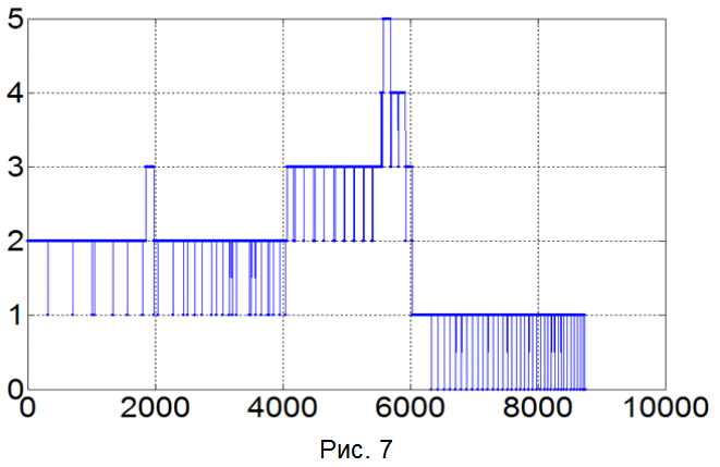
In Figure 7, we have a graph of the stack population, but in normal coordinates. A video illustrating the filling of the paw with a new color is offered below. It is made the same way - 50 frames per second.
As we see in this case, our stack (Fig. 7) turns out to be negligibly filled throughout the entire fill, and even with speed we won due to the search with a smaller depth.
Conclusion
In conclusion, I want to say - illustrate everything, even such simple algorithms, because there is power in beauty .
Also forgive forgiveness for a long article and as a seed for perhaps the next
Article cite the link . It describes another very interesting and very fast algorithm for filling me unfamiliar to this. Perhaps there is a hero with free time, who will also analyze this algorithm in detail and with illustrations.
And if someone has more powerful resources, then I propose to pour the belly of Carlson and put a video here, otherwise I have not enough patience while the video is being written. The blessing for this is all the code.
Used sources
Source: https://habr.com/ru/post/116374/
All Articles