Suffix array - a convenient replacement for the suffix tree
Hello, dear community! I think many people know such a data structure as a suffix tree . On Habré was already a description of how to build it and why. In short, it is necessary when it is necessary to look for arbitrary samples of X i in a predetermined text A many times, and such a tree is painfully constructed using the Ukkonen algorithm (there are other options, but they imply an even greater amount of suffering). The general observation when working with algorithms is such that trees are, of course, good, but in practice they are best avoided because of serious overheads from memory and not very optimal (in terms of the efficiency of operating data with a computer) location. In addition, it is in this tree that there is an even more significant nuisance, namely, the alphabetic dependence of the structure. To solve these problems, a suffix array was invented. About how to build it and how to use and go in this article.
The material of the article assumes knowledge of the concepts of the suffix and the string prefix , as well as knowledge of how binary search works. It is also necessary to imagine what is stable sorting and bitwise sorting , as well as understanding what is meant by stable sorting by counting. For some parts, we need knowledge of the minimum range problem - Range Minimum Query (RMQ) . Well, in general, you were warned: no one said it would be easy.
')
So, why doesn't a tree suit us? First, it is of course that due to the need to keep references to children, parents, etc. the size of the memory used in this case is noticeably larger than if these links are not stored. Secondly, if memory is allocated for data by some standard allocator, they will be “scattered in different corners,” as a result, bypassing the tree will involve a large number of memory transitions, which has a bad effect on the memory cache. Of course there are tricks that allow you to suppress this problem: you need to place the tree nodes in the array, and instead of pointers use the index in the array. Then the tree will be represented as a solid piece of memory.
Well, these are common problems for all trees. And what about the notorious alphabetical dependence? Let's look at the practical implementation of the suffix tree (if you have not encountered it, then it is not important to understand the essence of the problem). At each node of such a tree, there may be references to children in an amount of from 1 (for example, for a terminal vertex without branching) and up to the size of the alphabet. So the question is how to store these links. You can, for example, hold an array of links the size of the alphabet in each node. It will work quickly - to find out if there is an appropriate child in this node, it is possible for O (1). But in most cells of the array, zero references will be stored, and the memory will go to these cells. For small alphabets (for example, nucleotides in DNA) the hell with him, but imagine the Chinese characters? In principle, you don’t need to go far: not even the case-sensitive Russian alphabet makes you wonder if we want to have so much empty data.
It is possible to save memory more economically by placing only non-empty references in a dynamically changeable array (vector), but then checking for the presence of the corresponding node child for O (1) becomes quite doubtful. If you store links in sorted form, then O (log (size of the alphabet)). You can try to play with hash tables, but this will only make sense for very large alphabets, and also another level of indirection is introduced. And to build such trees is no longer O (n). In general, in any case, it will be necessary to make a compromise between memory and performance.
In 1989, Manber and Myers published an article in which they described such a data structure as a suffix array, and how to use it to search for substrings. A suffix array is an array of lexicographically sorted suffix strings (if the terminology is unfamiliar, then you can take a look at the “problem statement” section in this article). Generally speaking, there is no sense to keep the suffixes themselves; it is enough to keep the position of the beginning of the given suffix, but the definition of an array is so easily accepted. Here is an example for the mississippi line:
Also an important concept is the rank of the suffix - the place that the suffix will take when sorting, that is, its position in the suffix array. These are reciprocal values. We will not distinguish them in any way, since having one array, you can get another in O (N), so you can always have both on hand.

Consider an example. The original string "mississippi" . Suppose a sample comes to us "sip" . The easiest way to find out if a pattern is found in the text, using the suffix array, is to take the first character of the sample and use the binary search (the array is sorted) to find a range with suffixes starting with the same letter. Since all elements in the range are sorted, and the first characters are the same, the suffixes left after discarding the first character are also sorted. So, you can repeat the procedure of narrowing the search range to obtain either an empty range, or successful finding of all the characters of the sample. Obviously, in this way, in O (| X | log | A |) operations we will get the answer.
Exactly the same complexity will be obtained if we apply a binary search "in the forehead": with full lexicographic comparisons of strings along the edges and in the median with the sample: O (log | A |) comparisons with the average "price" of the comparison O (| X |).
Not bad, but better. In fact, it is not necessary to compare the entire search string with the element of the array. At each iteration of the binary search, we specify a certain range within which the desired element may be located. All strings in this range are somewhat similar. Namely, these strings may have a common prefix with the search string, since those that remained out of range will certainly not have a common prefix (in the sense that we do not consider the already processed part of the sample as part of the prefix).
Suppose we know the length of the common prefix of the remaining sample with the edges of the current range l = lcp ( X , S [ L ] ) and r = lcp ( X , S [ R ] ) for the left and right edges ( lcp - longest common prefix). The first statement is that for any string within the lcp range, it is no less than the minimum of these two numbers. If this were not so, then with the initial part of the prefix unchanged, there would be a position where the symbol would first coincide with the corresponding sample symbol, then not match, and then again match. This would contradict the sorting range. It is important to penetrate this idea well, as we will use it further for granted. The second statement is obvious: if the common prefix of the sample and any string within the range is not less than m = min (l, r), then m symbols can be skipped right away, knowing that they are the same in any case, and only be compared starting with m + 1 (and resulting in lcp for the given string).
Thus, we apply an optimized string comparison in a binary search for the head-on string. In the worst case, of course, we won’t gain anything from it: if the element we are looking for is on the edge of the array, but the neighbors are not at all similar to lcp, then r (or l) will be small each time, m will be small too, which means we will have to check each symbol by log | A | time. But experimental observations indicate that for natural texts, the search time is significantly reduced compared to O (log | A || X |), although it is difficult to assert anything about any particular asymptotics.
In principle, for practical applications this is quite enough, but if you want to squeeze everything, then ...
This is not the limit. The positions of the edges of a section of an array define the center of this section, and all such configurations that are realized in a binary search are a subset of a fixed set of size | A | -2. Suppose we have taken care to calculate in these configurations the values of m l = lcp ( S [ M ] , S [ L ] ) and m r = lcp ( S [ M ] , S [ R ] ), where M is the midpoint between L and R , in which we will go to the binary search step.
Let's look at one of the edges, say, left. If l <m l counted by us, then the left edge is similar to the middle (and to any element between them) much more than we would like, and then the result of the comparison is known in advance for the entire segment between L and M: lcp ( X , S [ M ] ) = l. From this it is immediately clear that the desired element is definitely not on this site, and if we look for it, then in the opposite half. If l> m l , then the middle is similar to the left edge less than the desired sample. So lcp ( X , S [ M ] ) = m l l , and the desired element should be found somewhere between them.
Naturally, nothing changes in the arguments, if we replace the left edge with the right one. Only one case was not considered: l = m l and r = m r (if at least one equality is not true, then the result is known according to the previous paragraph). Then it is clear that lcp ( X , S [ M ] ) is not less than max (l, r), but in order to determine it precisely and find out which way to go, it will be necessary to compare characters (finally!) Starting from the position max (l, r ) +1.
What have we got? We will do some steps of the binary search by comparing several lcp with each other, and even if it comes to comparing characters, then no more than once per character X (we take max (l, r) +1, which means we never go back). Thus, we obtain the complexity of the algorithm O (log | A | + | X |) in the worst case . True, we need pre-calculated lcp for text suffixes A found in the search tree induced by the binary search algorithm.
It is important to note that if we do not know m r , but only m l , then there is nothing terrible either. We lose the opportunity to say in advance that there is no entry, but this does not worsen the complexity: we just will not look at the right edge, only the left. If l <m l , then we search further in the other half, and l is saved, if l> m l , then r is taken as m l and we search in this half, and if l = m l , then we compare the median element with the required line starting with l + 1st position. We are not going back again in this case either, which means we can do without lcp for the left edges without degrading the complexity of the algorithm.
As you remember, in order to efficiently search for substrings we needed pre-calculated lcp for certain combinations of suffixes. It is necessary to explain how to get them. Methods are usually reduced to the task of finding the minimum in the segment - RMQ, so the algorithmic complexity of the algorithm is mostly determined by how effectively you can solve the RMQ problem. A more or less simple algorithm will cost O (NlogN) on preprocessing and O (1) on request. That is, if you use the construction of the suffix array for O (NlogN), then it is quite possible to use it. Of course, if you want to build a suffix array in linear time, you will have to apply the RMQ preprocessing algorithm in linear time with constant queries.
First, we build a so-called lcp-array - this is an array of lcp values between lexicographically-neighboring suffixes (after we have a suffix array, what suffixes do we have next-door questions). If we have an lcp-array, then finding lcp between two elements is reduced to finding the minimum value on a given segment of the lcp-array, that is, the task RMQ - finding the minimum on the segment - in its pure form. Why this is so is clear from considerations of the ordering of suffixes: if lcp between two lines were longer, then all the lines between them would also contain at least the same number of identical characters at the beginning, and all lcp between these lines would be no less than mutual lcp items.
Building an lcp array is quite simple. Of course, it is impossible to go along the suffix array and count lcp neighboring elements - this is O (N 2 ). But if you go through the array in the correct order, you can use the information from the previous step for calculations. Namely, if we iterate suffixes in the order in which they appear in the source line, then at each step lcp cannot be reduced by more than 1 compared to the previous step, that is, it can be more, it may not change, but if less, only by 1. This happens for the following reason. If you find out that lcp ( A [i ..], A [j ..]) = l, then discarding the first character obviously reduces it by one: lcp ( A [i + 1 ..], A [j +1 ..]) = l-1. Of course, if the i-th and j-th suffixes turned out to be lexicographically adjacent, then this does not guarantee that i + 1-st and j + 1-th will be adjacent - between them, most likely, others will interpose. But, as we have already found out, lcp between them is the minimum lcp on the whole segment between them, which means lcp between the i + 1th suffix and the lexicographically following it is not less than l-1.
This allows you to skip all the characters to the last but one (l-1), since we are sure that they are equal, and only compare the l-th character and beyond. This means that any checks we made either increase the current lcp, or force us to move to the next iteration. Thus, having passed all suffixes except the lexicographically last (it must be skipped), we get an lcp-array in linear time O (N).
Well that's all. It remains to find the RMQ for the pairs of suffixes we need. The RMQ solution consists of preprocessing and, in fact, responses to requests for a minimum between the elements. Since the main computational load falls on preprocessing, and query execution can be done O (1), generally speaking it is not necessary to explicitly write the pairs of interest and lcp between them, since we can answer about O lcp of an arbitrary pair of suffixes in O (1) including those that play a role in a binary search. Given that this eliminates the need to think about how to address stored values, this is very cool. If you still want to store lcp in an already counted form, then you need to correctly number the states in the search tree - read about the location in memory and addressing in the binary heap.
I will not write about how to solve RMQ - on Habré there was already a good article about a simple version for O (NlogN), and I hope there will be a continuation in which they will write about a hardcore version for O (N) - Farah-Colton algorithm and Bender .
Great, here we know how to apply a suffix array, but where does it come from? Obviously, building it in a direct way, sorting suffixes, is a long matter - O (N 2 logN), where N = | A |. There are a number of algorithms that work for O (NlogN), there are those that work for O (N). Those that are O (N) are very complicated (for example, first constructing a suffix tree, and then from it already collect a suffix array). If the maximum efficiency in a specific task is not so important, then you should think about the clarity of the code and stop at the NlogN option. Next, go one traversal algorithm from these categories.
Recall how bitwise sorting works: first, we distribute items into baskets (buckets) by counting based on the low-order bit, then we do the same with the next digit, etc. Here we will act in a similar way, but still a bit differently - if we directly apply the bitwise sorting to suffixes, then we get O (N 2 ).
Suppose that at some step we sorted (more precisely, arranged on baskets - buckets) lines according to H first characters. We can number these parts of the rows by their basket numbers. But each suffix S [ i ] = A [ i .. ] is found not only as an element of the array, but also as part of other elements of the array, in particular as a substring in the H position of the suffix S [ iH ] (omit for clarity, the edge effects lines - they can be bypassed by writing down at the end of the desired number of centilenes) That is, having numbered the first H characters of suffixes with the numbers of baskets, we automatically enumerate the second H characters. Then we get a set of pairs consisting of basket numbers (of some step). Having sorted these pairs by bitwise sorting, we will get O (N) strings, strung in baskets by 2H first characters. Thus, the number of characters processed at each step will double. This gives O (logN) steps and the overall complexity of the O (NlogN) algorithm.

Another small note regarding the first step. If in the next steps we have to sort the numbers of the baskets, which does not cause problems with the bitwise sorting, then the first step is to sort the lines by the first character. Depending on the nature of the alphabet, it may turn out that it is impossible to apply bitwise sorting there. Then you can apply any other sorting based on comparisons with O (NlogN) complexity, and find basket ranges for O (N). The overall complexity of the algorithm will not change this.
This is a fairly new algorithm, published in 2003 by Karkainen and Sanders. Immediately I will warn you that this algorithm works only on alphabets, the characters of which can be numbered in O (N) time (it is equivalent to sort the numbers, that is, you need to know how to sort by O (N) bitwise sorting). Other is rare, but still happens.
The algorithm is recursive, that is, at some stage we get the same problem of finding the suffix array for a string of shorter length. Consider the mississippi example. So, the first thing we will do is enumerate our characters in numbers from 1 to N, going to the numerical alphabet. As we mentioned, this can be done using O (N) bitwise sorting. After that, the original "real" characters do not interest us, we work only with a numeric representation of the string. You can forget that this was once not a numeric sequence.
Next, we want to build a superalphabet that will contain all the trigrams in the text, and again number the characters of this new alphabet in lexicographical order. It is clear that these trigrams are no more than characters in a string (less, if there are coinciding). Since we want to be able to work effectively with this alphabet, the option to look for a trigram in a superalphabet every time and return its lexicographic position (the lexicographic position is sometimes also called rank) does not roll. We must immediately numbered the superscript, so that questions about this trigram would not arise at all. For this, it is necessary to match each character of the input string (is it numeric, have you not forgotten?) The number of the trigram in this position. This is done by a bitwise sorting of all trigrams (together with duplicates) from the source line, preserving what position the trigram came from. Subsequent numbering in this case is not difficult.
For example, from A = "mississippi" one can get trigrams {mis, iss, ssi, ... ppi, pi $, i $$}, and in lexicographical order {i $$, ipp, iss, ... ssi}. We have added a line as needed by the centinels and consider them to be minimal characters.
At this stage, it may turn out that all trigrams in the line are different. This can be used as an early terminal condition, since if trigrams are different, their lexicographic order sets the lexicographic order of the suffixes (you can not use this condition, but simply continue to reduce the string to a shorter one until the answer becomes obvious). We can present the original line in the form of trigrams in three ways: breaking the line itself into trigrams, a line without the first character and a line without the first two characters. We call these representations of the rows T 0 , T 1 and T 2 . Each of them is about three times shorter than the original. If you count positions from zero, then you can call these representations corresponding to the group of suffixes in positions i mod 3 = 0, i mod 3 = 1 and i mod 3 = 2.
Next, a feint is made with ears, the meaning of which will be clear later: we take two of these three lines, for concreteness, T 1 and T 2 , presented in the form of trigrams, concatenated and passed to the same algorithm in a recursive call. Obviously, the length of the transmitted string is one third shorter than the original. At the output of the algorithm, we expect a suffix array (or, equivalently, an array of ranks). Turning back from trigrams to a numeric string, we will receive information on the lexicographic order between the suffixes of groups 1 and 2.
The suffix of group 0 can be represented as a pair consisting of a symbol and a suffix of group 1, or as a triple of two symbols and a suffix of group 2: A [3k ..] = (A [3k], A [3k + 1 ..]) = (A [3k], A [3k + 1], A [3k + 2 ..]). Similar expressions can be written to translate other groups of suffixes into adjacent ones. We represent type 0 suffixes as a pair of a symbol and a type 1 suffix (more precisely, the type 1 suffix rank, we are not interested in the suffix), then sort them by bitwise sorting.
At this stage, we have the result of a recursive function call in the form of mutually sorted type 1 and 2 suffixes, and sorted type 0 suffixes. We need to merge them using the usual merging of sorted arrays, but at the same time we need to be able to effectively compare type 0 suffixes 1 and 2. In order to compare the type 0 suffix with type 1, you must convert the type 0 suffix to type 1, and type 1 to type 2: (A [3l], A [3l + 1 ..]) VS (A [3m + 1], A [3m + 2] ..). It is easy to compare these two pairs: either the first character determines the order, or if it is equal, then the order determines the order of the suffixes of groups 1 and 2, which we know from the results of the recursive call of this algorithm. For comparison of the suffix of types 0 and 2, the chain is slightly larger, but the essence is the same: (A [3l], A [3l + 1], A [3l + 2 ..]) VS (A [3m + 2], A [3 (m + 1)], A [3 (m + 1) +1 ..]).
At first glance, it is not clear why all this should give us a linear complexity. First, let's deal with everything except the recursive call. The superscript bitwise sorting, suffix marking is all O (N), bitwise sorting of group 0 suffixes and merging sorted arrays is also O (N). Now the recursive call - we call the algorithm 2/3 of the original length of the string, thus the complexity of the algorithm is T (N) = T (2N / 3) + O (N). If to paint this expression substituting it in itself, then we will receive the sum of a geometrical progression with coefficient 2/3, so limited O (N). The resulting complexity is thus O (N).
Here it is described how to apply the suffix array and how to build it. Algorithms are quite voluminous, but what to do is a very high-level task. I described it all in fairly general terms and did not provide any code for an understandable reason - then there would be too many words and code. As you can see, the algorithms are fast and a little slower differ significantly in implementation complexity, so there is a reason to think a few times whether you really need to do this, for example, for O (N), and not for O (NlogN).
I also anticipate questions like “where you can see the finished implementation,” “where to read more,” and so on. I haven’t seen any ready-made implementations in the “just add your comparator” style, although the wikipedia page claims that they exist. Here and here there are explanations and some implementation. In addition, in the original article by Karkainen and Sanders, there is also an array construction code. About NlogN construction can be read in the article Manber and Myers: Udi Manber, Gene Myers - "Suffix arrays: a new method for on-line string searches."
The material of the article assumes knowledge of the concepts of the suffix and the string prefix , as well as knowledge of how binary search works. It is also necessary to imagine what is stable sorting and bitwise sorting , as well as understanding what is meant by stable sorting by counting. For some parts, we need knowledge of the minimum range problem - Range Minimum Query (RMQ) . Well, in general, you were warned: no one said it would be easy.
')
Suffix array applications
Not all trees are equally useful.
So, why doesn't a tree suit us? First, it is of course that due to the need to keep references to children, parents, etc. the size of the memory used in this case is noticeably larger than if these links are not stored. Secondly, if memory is allocated for data by some standard allocator, they will be “scattered in different corners,” as a result, bypassing the tree will involve a large number of memory transitions, which has a bad effect on the memory cache. Of course there are tricks that allow you to suppress this problem: you need to place the tree nodes in the array, and instead of pointers use the index in the array. Then the tree will be represented as a solid piece of memory.
Well, these are common problems for all trees. And what about the notorious alphabetical dependence? Let's look at the practical implementation of the suffix tree (if you have not encountered it, then it is not important to understand the essence of the problem). At each node of such a tree, there may be references to children in an amount of from 1 (for example, for a terminal vertex without branching) and up to the size of the alphabet. So the question is how to store these links. You can, for example, hold an array of links the size of the alphabet in each node. It will work quickly - to find out if there is an appropriate child in this node, it is possible for O (1). But in most cells of the array, zero references will be stored, and the memory will go to these cells. For small alphabets (for example, nucleotides in DNA) the hell with him, but imagine the Chinese characters? In principle, you don’t need to go far: not even the case-sensitive Russian alphabet makes you wonder if we want to have so much empty data.
It is possible to save memory more economically by placing only non-empty references in a dynamically changeable array (vector), but then checking for the presence of the corresponding node child for O (1) becomes quite doubtful. If you store links in sorted form, then O (log (size of the alphabet)). You can try to play with hash tables, but this will only make sense for very large alphabets, and also another level of indirection is introduced. And to build such trees is no longer O (n). In general, in any case, it will be necessary to make a compromise between memory and performance.
Suffix array
In 1989, Manber and Myers published an article in which they described such a data structure as a suffix array, and how to use it to search for substrings. A suffix array is an array of lexicographically sorted suffix strings (if the terminology is unfamiliar, then you can take a look at the “problem statement” section in this article). Generally speaking, there is no sense to keep the suffixes themselves; it is enough to keep the position of the beginning of the given suffix, but the definition of an array is so easily accepted. Here is an example for the mississippi line:
| # | suffix | suffix number |
|---|---|---|
| one | i | eleven |
| 2 | ippi | eight |
| 3 | issippi | five |
| four | ississippi | 2 |
| five | mississippi | one |
| 6 | pi | ten |
| 7 | ppi | 9 |
| eight | sippi | 7 |
| 9 | sissippi | four |
| ten | ssippi | 6 |
| eleven | ssissippi | 3 |
Also an important concept is the rank of the suffix - the place that the suffix will take when sorting, that is, its position in the suffix array. These are reciprocal values. We will not distinguish them in any way, since having one array, you can get another in O (N), so you can always have both on hand.
Simplest substring search
Consider an example. The original string "mississippi" . Suppose a sample comes to us "sip" . The easiest way to find out if a pattern is found in the text, using the suffix array, is to take the first character of the sample and use the binary search (the array is sorted) to find a range with suffixes starting with the same letter. Since all elements in the range are sorted, and the first characters are the same, the suffixes left after discarding the first character are also sorted. So, you can repeat the procedure of narrowing the search range to obtain either an empty range, or successful finding of all the characters of the sample. Obviously, in this way, in O (| X | log | A |) operations we will get the answer.
| sample | s ip | si p | sip |
|---|---|---|---|
| i | i | i | |
| ippi | ippi | ippi | |
| issippi | issippi | issippi | |
| ississippi | ississippi | ississippi | |
| mississippi | mississippi | mississippi | |
| pi | pi | pi | |
| ppi | ppi | ppi | |
| s ippi | si ppi | sip pi | |
| s issippi | si ssippi | sissippi | |
| s sippi | ssippi | ssippi | |
| s sissippi | ssissippi | ssissippi |
Exactly the same complexity will be obtained if we apply a binary search "in the forehead": with full lexicographic comparisons of strings along the edges and in the median with the sample: O (log | A |) comparisons with the average "price" of the comparison O (| X |).
Faster
Not bad, but better. In fact, it is not necessary to compare the entire search string with the element of the array. At each iteration of the binary search, we specify a certain range within which the desired element may be located. All strings in this range are somewhat similar. Namely, these strings may have a common prefix with the search string, since those that remained out of range will certainly not have a common prefix (in the sense that we do not consider the already processed part of the sample as part of the prefix).
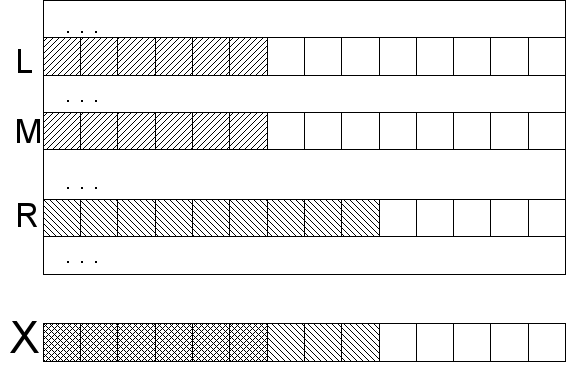
Suppose we know the length of the common prefix of the remaining sample with the edges of the current range l = lcp ( X , S [ L ] ) and r = lcp ( X , S [ R ] ) for the left and right edges ( lcp - longest common prefix). The first statement is that for any string within the lcp range, it is no less than the minimum of these two numbers. If this were not so, then with the initial part of the prefix unchanged, there would be a position where the symbol would first coincide with the corresponding sample symbol, then not match, and then again match. This would contradict the sorting range. It is important to penetrate this idea well, as we will use it further for granted. The second statement is obvious: if the common prefix of the sample and any string within the range is not less than m = min (l, r), then m symbols can be skipped right away, knowing that they are the same in any case, and only be compared starting with m + 1 (and resulting in lcp for the given string).
Thus, we apply an optimized string comparison in a binary search for the head-on string. In the worst case, of course, we won’t gain anything from it: if the element we are looking for is on the edge of the array, but the neighbors are not at all similar to lcp, then r (or l) will be small each time, m will be small too, which means we will have to check each symbol by log | A | time. But experimental observations indicate that for natural texts, the search time is significantly reduced compared to O (log | A || X |), although it is difficult to assert anything about any particular asymptotics.
In principle, for practical applications this is quite enough, but if you want to squeeze everything, then ...
Even faster
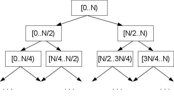
This is not the limit. The positions of the edges of a section of an array define the center of this section, and all such configurations that are realized in a binary search are a subset of a fixed set of size | A | -2. Suppose we have taken care to calculate in these configurations the values of m l = lcp ( S [ M ] , S [ L ] ) and m r = lcp ( S [ M ] , S [ R ] ), where M is the midpoint between L and R , in which we will go to the binary search step.
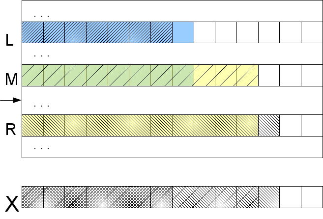
Let's look at one of the edges, say, left. If l <m l counted by us, then the left edge is similar to the middle (and to any element between them) much more than we would like, and then the result of the comparison is known in advance for the entire segment between L and M: lcp ( X , S [ M ] ) = l. From this it is immediately clear that the desired element is definitely not on this site, and if we look for it, then in the opposite half. If l> m l , then the middle is similar to the left edge less than the desired sample. So lcp ( X , S [ M ] ) = m l l , and the desired element should be found somewhere between them.
Naturally, nothing changes in the arguments, if we replace the left edge with the right one. Only one case was not considered: l = m l and r = m r (if at least one equality is not true, then the result is known according to the previous paragraph). Then it is clear that lcp ( X , S [ M ] ) is not less than max (l, r), but in order to determine it precisely and find out which way to go, it will be necessary to compare characters (finally!) Starting from the position max (l, r ) +1.
What have we got? We will do some steps of the binary search by comparing several lcp with each other, and even if it comes to comparing characters, then no more than once per character X (we take max (l, r) +1, which means we never go back). Thus, we obtain the complexity of the algorithm O (log | A | + | X |) in the worst case . True, we need pre-calculated lcp for text suffixes A found in the search tree induced by the binary search algorithm.
It is important to note that if we do not know m r , but only m l , then there is nothing terrible either. We lose the opportunity to say in advance that there is no entry, but this does not worsen the complexity: we just will not look at the right edge, only the left. If l <m l , then we search further in the other half, and l is saved, if l> m l , then r is taken as m l and we search in this half, and if l = m l , then we compare the median element with the required line starting with l + 1st position. We are not going back again in this case either, which means we can do without lcp for the left edges without degrading the complexity of the algorithm.
LCP pretreatment
As you remember, in order to efficiently search for substrings we needed pre-calculated lcp for certain combinations of suffixes. It is necessary to explain how to get them. Methods are usually reduced to the task of finding the minimum in the segment - RMQ, so the algorithmic complexity of the algorithm is mostly determined by how effectively you can solve the RMQ problem. A more or less simple algorithm will cost O (NlogN) on preprocessing and O (1) on request. That is, if you use the construction of the suffix array for O (NlogN), then it is quite possible to use it. Of course, if you want to build a suffix array in linear time, you will have to apply the RMQ preprocessing algorithm in linear time with constant queries.
First, we build a so-called lcp-array - this is an array of lcp values between lexicographically-neighboring suffixes (after we have a suffix array, what suffixes do we have next-door questions). If we have an lcp-array, then finding lcp between two elements is reduced to finding the minimum value on a given segment of the lcp-array, that is, the task RMQ - finding the minimum on the segment - in its pure form. Why this is so is clear from considerations of the ordering of suffixes: if lcp between two lines were longer, then all the lines between them would also contain at least the same number of identical characters at the beginning, and all lcp between these lines would be no less than mutual lcp items.
Building an lcp array is quite simple. Of course, it is impossible to go along the suffix array and count lcp neighboring elements - this is O (N 2 ). But if you go through the array in the correct order, you can use the information from the previous step for calculations. Namely, if we iterate suffixes in the order in which they appear in the source line, then at each step lcp cannot be reduced by more than 1 compared to the previous step, that is, it can be more, it may not change, but if less, only by 1. This happens for the following reason. If you find out that lcp ( A [i ..], A [j ..]) = l, then discarding the first character obviously reduces it by one: lcp ( A [i + 1 ..], A [j +1 ..]) = l-1. Of course, if the i-th and j-th suffixes turned out to be lexicographically adjacent, then this does not guarantee that i + 1-st and j + 1-th will be adjacent - between them, most likely, others will interpose. But, as we have already found out, lcp between them is the minimum lcp on the whole segment between them, which means lcp between the i + 1th suffix and the lexicographically following it is not less than l-1.
| # | suffix | step | lcp |
|---|---|---|---|
| one | i | ten | one |
| 2 | ippi | 7 | one |
| 3 | issippi | four | four |
| four | ississippi | 2 | 0 |
| five | mississippi | one | 0 |
| 6 | pi | 9 | one |
| 7 | ppi | eight | 0 |
| eight | sippi | 6 | 2 |
| 9 | sissippi | 3 | one |
| ten | ssippi | five | 3 |
| eleven | ssissippi | skip |
This allows you to skip all the characters to the last but one (l-1), since we are sure that they are equal, and only compare the l-th character and beyond. This means that any checks we made either increase the current lcp, or force us to move to the next iteration. Thus, having passed all suffixes except the lexicographically last (it must be skipped), we get an lcp-array in linear time O (N).
Well that's all. It remains to find the RMQ for the pairs of suffixes we need. The RMQ solution consists of preprocessing and, in fact, responses to requests for a minimum between the elements. Since the main computational load falls on preprocessing, and query execution can be done O (1), generally speaking it is not necessary to explicitly write the pairs of interest and lcp between them, since we can answer about O lcp of an arbitrary pair of suffixes in O (1) including those that play a role in a binary search. Given that this eliminates the need to think about how to address stored values, this is very cool. If you still want to store lcp in an already counted form, then you need to correctly number the states in the search tree - read about the location in memory and addressing in the binary heap.
I will not write about how to solve RMQ - on Habré there was already a good article about a simple version for O (NlogN), and I hope there will be a continuation in which they will write about a hardcore version for O (N) - Farah-Colton algorithm and Bender .
Building a suffix array
Great, here we know how to apply a suffix array, but where does it come from? Obviously, building it in a direct way, sorting suffixes, is a long matter - O (N 2 logN), where N = | A |. There are a number of algorithms that work for O (NlogN), there are those that work for O (N). Those that are O (N) are very complicated (for example, first constructing a suffix tree, and then from it already collect a suffix array). If the maximum efficiency in a specific task is not so important, then you should think about the clarity of the code and stop at the NlogN option. Next, go one traversal algorithm from these categories.
Over O (NlogN)
Recall how bitwise sorting works: first, we distribute items into baskets (buckets) by counting based on the low-order bit, then we do the same with the next digit, etc. Here we will act in a similar way, but still a bit differently - if we directly apply the bitwise sorting to suffixes, then we get O (N 2 ).
Suppose that at some step we sorted (more precisely, arranged on baskets - buckets) lines according to H first characters. We can number these parts of the rows by their basket numbers. But each suffix S [ i ] = A [ i .. ] is found not only as an element of the array, but also as part of other elements of the array, in particular as a substring in the H position of the suffix S [ iH ] (omit for clarity, the edge effects lines - they can be bypassed by writing down at the end of the desired number of centilenes) That is, having numbered the first H characters of suffixes with the numbers of baskets, we automatically enumerate the second H characters. Then we get a set of pairs consisting of basket numbers (of some step). Having sorted these pairs by bitwise sorting, we will get O (N) strings, strung in baskets by 2H first characters. Thus, the number of characters processed at each step will double. This gives O (logN) steps and the overall complexity of the O (NlogN) algorithm.
Another small note regarding the first step. If in the next steps we have to sort the numbers of the baskets, which does not cause problems with the bitwise sorting, then the first step is to sort the lines by the first character. Depending on the nature of the alphabet, it may turn out that it is impossible to apply bitwise sorting there. Then you can apply any other sorting based on comparisons with O (NlogN) complexity, and find basket ranges for O (N). The overall complexity of the algorithm will not change this.
Over O (N)
This is a fairly new algorithm, published in 2003 by Karkainen and Sanders. Immediately I will warn you that this algorithm works only on alphabets, the characters of which can be numbered in O (N) time (it is equivalent to sort the numbers, that is, you need to know how to sort by O (N) bitwise sorting). Other is rare, but still happens.
The algorithm is recursive, that is, at some stage we get the same problem of finding the suffix array for a string of shorter length. Consider the mississippi example. So, the first thing we will do is enumerate our characters in numbers from 1 to N, going to the numerical alphabet. As we mentioned, this can be done using O (N) bitwise sorting. After that, the original "real" characters do not interest us, we work only with a numeric representation of the string. You can forget that this was once not a numeric sequence.
Next, we want to build a superalphabet that will contain all the trigrams in the text, and again number the characters of this new alphabet in lexicographical order. It is clear that these trigrams are no more than characters in a string (less, if there are coinciding). Since we want to be able to work effectively with this alphabet, the option to look for a trigram in a superalphabet every time and return its lexicographic position (the lexicographic position is sometimes also called rank) does not roll. We must immediately numbered the superscript, so that questions about this trigram would not arise at all. For this, it is necessary to match each character of the input string (is it numeric, have you not forgotten?) The number of the trigram in this position. This is done by a bitwise sorting of all trigrams (together with duplicates) from the source line, preserving what position the trigram came from. Subsequent numbering in this case is not difficult.
For example, from A = "mississippi" one can get trigrams {mis, iss, ssi, ... ppi, pi $, i $$}, and in lexicographical order {i $$, ipp, iss, ... ssi}. We have added a line as needed by the centinels and consider them to be minimal characters.
| original line: | m | i | s | s | i | s | s | i | p | p | i |
| numeric string: | 2 | one | four | four | one | four | four | one | 3 | 3 | one |
| trigrams: | mis | iss | ssi | sis | iss | ssi | sip | ipp | ppi | pi $ | i $$ |
| trigram numbering: | four | 3 | 9 | eight | 3 | 9 | 7 | 2 | 6 | five | one |
At this stage, it may turn out that all trigrams in the line are different. This can be used as an early terminal condition, since if trigrams are different, their lexicographic order sets the lexicographic order of the suffixes (you can not use this condition, but simply continue to reduce the string to a shorter one until the answer becomes obvious). We can present the original line in the form of trigrams in three ways: breaking the line itself into trigrams, a line without the first character and a line without the first two characters. We call these representations of the rows T 0 , T 1 and T 2 . Each of them is about three times shorter than the original. If you count positions from zero, then you can call these representations corresponding to the group of suffixes in positions i mod 3 = 0, i mod 3 = 1 and i mod 3 = 2.
| T 0 : | mis | sis | sip | pi $ |
| four | eight | 7 | five | |
| T 1 : | iss | iss | ipp | i $$ |
| 3 | 3 | 2 | one | |
| T 2 : | ssi | ssi | ppi | |
| 9 | 9 | 6 |
Next, a feint is made with ears, the meaning of which will be clear later: we take two of these three lines, for concreteness, T 1 and T 2 , presented in the form of trigrams, concatenated and passed to the same algorithm in a recursive call. Obviously, the length of the transmitted string is one third shorter than the original. At the output of the algorithm, we expect a suffix array (or, equivalently, an array of ranks). Turning back from trigrams to a numeric string, we will receive information on the lexicographic order between the suffixes of groups 1 and 2.
The suffix of group 0 can be represented as a pair consisting of a symbol and a suffix of group 1, or as a triple of two symbols and a suffix of group 2: A [3k ..] = (A [3k], A [3k + 1 ..]) = (A [3k], A [3k + 1], A [3k + 2 ..]). Similar expressions can be written to translate other groups of suffixes into adjacent ones. We represent type 0 suffixes as a pair of a symbol and a type 1 suffix (more precisely, the type 1 suffix rank, we are not interested in the suffix), then sort them by bitwise sorting.
At this stage, we have the result of a recursive function call in the form of mutually sorted type 1 and 2 suffixes, and sorted type 0 suffixes. We need to merge them using the usual merging of sorted arrays, but at the same time we need to be able to effectively compare type 0 suffixes 1 and 2. In order to compare the type 0 suffix with type 1, you must convert the type 0 suffix to type 1, and type 1 to type 2: (A [3l], A [3l + 1 ..]) VS (A [3m + 1], A [3m + 2] ..). It is easy to compare these two pairs: either the first character determines the order, or if it is equal, then the order determines the order of the suffixes of groups 1 and 2, which we know from the results of the recursive call of this algorithm. For comparison of the suffix of types 0 and 2, the chain is slightly larger, but the essence is the same: (A [3l], A [3l + 1], A [3l + 2 ..]) VS (A [3m + 2], A [3 (m + 1)], A [3 (m + 1) +1 ..]).
At first glance, it is not clear why all this should give us a linear complexity. First, let's deal with everything except the recursive call. The superscript bitwise sorting, suffix marking is all O (N), bitwise sorting of group 0 suffixes and merging sorted arrays is also O (N). Now the recursive call - we call the algorithm 2/3 of the original length of the string, thus the complexity of the algorithm is T (N) = T (2N / 3) + O (N). If to paint this expression substituting it in itself, then we will receive the sum of a geometrical progression with coefficient 2/3, so limited O (N). The resulting complexity is thus O (N).
Conclusion
Here it is described how to apply the suffix array and how to build it. Algorithms are quite voluminous, but what to do is a very high-level task. I described it all in fairly general terms and did not provide any code for an understandable reason - then there would be too many words and code. As you can see, the algorithms are fast and a little slower differ significantly in implementation complexity, so there is a reason to think a few times whether you really need to do this, for example, for O (N), and not for O (NlogN).
I also anticipate questions like “where you can see the finished implementation,” “where to read more,” and so on. I haven’t seen any ready-made implementations in the “just add your comparator” style, although the wikipedia page claims that they exist. Here and here there are explanations and some implementation. In addition, in the original article by Karkainen and Sanders, there is also an array construction code. About NlogN construction can be read in the article Manber and Myers: Udi Manber, Gene Myers - "Suffix arrays: a new method for on-line string searches."
Source: https://habr.com/ru/post/115346/
All Articles