Commentary on the Canni Outline Algorithm

annotation

In the article Canny Boundaries Detector , as I already wrote in the comments to it, the algorithm essence is distorted and lost in the place where the search for the gradient occurs. To do this, it uses the core of Sobel, about which Kanni did not say anything at all. I wrote an amendment that will allow the contour extraction algorithm to work faster. Also, this article can be considered a continuation of the recording of the image gradient .
The article does not deal with the choice of the optimal discretization step of the lubrication core.

Prerequisites

1. Before the gradient of the image brightness function is calculated, it is often necessary to filter noise using a Gaussian filter to obtain a stable result, that is, a preliminary blur is performed.
2. Then, using differential approximations of the derivatives, the components of the gradient are found.

Let lubrication be done using a kernel with the size of NxN points, and differential patterns for calculating derivatives along the axes are 1xK and Kx1 . The size of the image is set equal to MxM .
For simplicity, we will only consider multiplications, then the sequence “Lubricant-> Gradient” will require N ^ 2 * M ^ 2 + 2 * K * M ^ 2 = (N ^ 2 + 2 * K) * M ^ 2 operations.

However, the formula is known

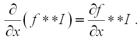
the use of which will allow us to reduce the number of orders of magnitude. What is she talking about? - that, in principle, it is not necessary to first perform the lubrication and then differentiate the image. You can differentiate the kernel of blurring f and then perform the convolution. Let's get started

Core separation

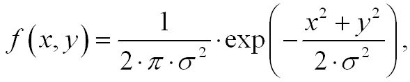
Let's look at the two-dimensional Gauss function:

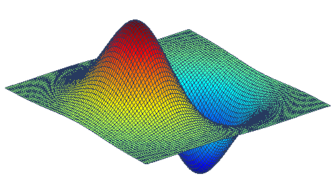
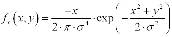
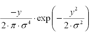
its derivative with respect to x is written as:

We can get this wonderful derivative by executing the MatLab code:
sigma = 1.4; x = -3*sigma:0.1:3*sigma y = x; [x,y] = meshgrid(x,y); Fx1 = ( -x/2/pi/sigma^2 ).*exp( -(x.^2+y.^2)/2/sigma^2 ); figure; surf(Fx1) * This source code was highlighted with Source Code Highlighter .


1. sigma = 1.4; x = -3*sigma:0.1:3*sigma y = x; [x,y] = meshgrid(x,y); Fx1 = ( -x/2/pi/sigma^2 ).*exp( -(x.^2+y.^2)/2/sigma^2 ); figure; surf(Fx1) * This source code was highlighted with Source Code Highlighter .

2. sigma = 1.4; x = -3*sigma:0.1:3*sigma y = x; [x,y] = meshgrid(x,y); Fx1 = ( -x/2/pi/sigma^2 ).*exp( -(x.^2+y.^2)/2/sigma^2 ); figure; surf(Fx1) * This source code was highlighted with Source Code Highlighter .

3. sigma = 1.4; x = -3*sigma:0.1:3*sigma y = x; [x,y] = meshgrid(x,y); Fx1 = ( -x/2/pi/sigma^2 ).*exp( -(x.^2+y.^2)/2/sigma^2 ); figure; surf(Fx1) * This source code was highlighted with Source Code Highlighter .

4. sigma = 1.4; x = -3*sigma:0.1:3*sigma y = x; [x,y] = meshgrid(x,y); Fx1 = ( -x/2/pi/sigma^2 ).*exp( -(x.^2+y.^2)/2/sigma^2 ); figure; surf(Fx1) * This source code was highlighted with Source Code Highlighter .

5. sigma = 1.4; x = -3*sigma:0.1:3*sigma y = x; [x,y] = meshgrid(x,y); Fx1 = ( -x/2/pi/sigma^2 ).*exp( -(x.^2+y.^2)/2/sigma^2 ); figure; surf(Fx1) * This source code was highlighted with Source Code Highlighter .

6. sigma = 1.4; x = -3*sigma:0.1:3*sigma y = x; [x,y] = meshgrid(x,y); Fx1 = ( -x/2/pi/sigma^2 ).*exp( -(x.^2+y.^2)/2/sigma^2 ); figure; surf(Fx1) * This source code was highlighted with Source Code Highlighter .


sigma = 1.4; x = -3*sigma:0.1:3*sigma y = x; [x,y] = meshgrid(x,y); Fx1 = ( -x/2/pi/sigma^2 ).*exp( -(x.^2+y.^2)/2/sigma^2 ); figure; surf(Fx1) * This source code was highlighted with Source Code Highlighter .


sigma = 1.4; x = -3*sigma:0.1:3*sigma y = x; [x,y] = meshgrid(x,y); Fx1 = ( -x/2/pi/sigma^2 ).*exp( -(x.^2+y.^2)/2/sigma^2 ); figure; surf(Fx1) * This source code was highlighted with Source Code Highlighter .

A filter with such a kernel is sometimes called a Canny filter, and a kernel is called a Canny kernel, which, like other operators, approximates a derivative. On this occasion, I share a remarkably illustrated note .
')
Note that the derivative is separable by coordinates, which means we can implement a row-column algorithm for calculating a blurred image gradient:

Calculate the number of operations in the case of a string-column algorithm.

To obtain the derivative with respect to y:

1. We process the Gauss image I in rows with a 1xK1 window, get the image I1 for K * M ^ 2 multiplications (Don't forget to normalize the kernel),
2. We process the image I1 in rows with a core of size K1x1 :
   
   
   
   (Do not forget to select the core sampling steps so that the sum of samples is 0)
   For such an operation, we need the same - K * M ^ 2 multiplications.
   

The algorithm for deriving the derivative with respect to x is similar, and summing up the number of operations we get that to calculate the components of the blurred gradient we need 4 * K1 * M ^ 2.

Efficiency

The effectiveness of the described optimization can be quantitatively expressed by the relation:

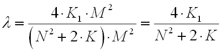
It turned out that efficiency depends only on the size of the windows, but not on the size of the images.
Suppose that in a simple algorithm the kernel of size N = 5 is used for blurring, and for calculating derivatives, the first order approximation (kernels [-1 1] and [-1 1] ') is K = 2.

In the case of an optimized row-column algorithm, we set K1 = 5. Then λ = 20/29 = 0.68.
Efficiency λ <1 - we managed to reduce the number of arithmetic operations when calculating the Smaz-Gradient sequence.