Canny Boundary Detector
Good day!
Recently, on Habré, Kanni’s border selection algorithm (which, to my surprise, translates literally: tricky) has often been mentioned. So, I matured to share with the public my experience in implementing this detector.
In my spare time, in order to educate myself, I study algorithms (including machine vision). I deal with this unprofessionally, in many respects adhering to popular scientific literature or my own algorithmic solutions.
On the one hand, to simplify coding, and on the other hand, to give a narration to a note of brainfuck programming, I will show implementation in the Mathcad computer algebra environment (algorithms tested in versions 13 and 14), with as little as possible using specific built-in methods. Such a campaign, in my opinion, improves the perception of the demonstration, and facilitates the possible transfer of algorithms to other design / development environments. It should be noted that some stages of the Kanni detector operation may involve not only various optimization (for example, software implementation of the Sobel operator using SIMD-expansion of the processor command system), but also the possibility of replacing some operators (methods) with others (for example, the Sobel operator can be replaced operator Roberts or Pruitt), and the possibility of varying the coefficients that define the parameters of the operators.
This version was created for reasons of maximum ease of implementation in the Mathcad environment, possibly at the expense of performance in terms of speed and quality of detection, and is presented as a demonstration of the main stages of the functioning of the Canny detector.
Kanni (John F. Canny; 1953) studied the mathematical problem of obtaining a filter that is optimal according to the criteria for isolating, localizing and minimizing several responses of one edge. This means that the detector should react to the borders, but at the same time ignore the false ones, accurately determine the border line (without fragmenting it) and respond to each border once, thus avoiding the perception of wide bands of brightness as a combination of borders. Kanni introduced the concept of Non-Maximum Suppression, which means that the pixels at the edges are declared at which the local maximum of the gradient in the direction of the gradient vector is reached.
Although his work was carried out at the dawn of computer vision (1986), Kanney's boundary detector is still one of the best detectors. In addition to particular special cases, it is difficult to find a detector that would work substantially better than the Kanni detector.
')
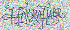
As a demonstration of the operation of the algorithm, the problem of boundary selection in the next image will be solved.
The algorithm consists of five separate steps:
To convert the original image into an image in grayscale, you need to get its "brightness" -component. For this, it is convenient to present the image in the YUV color model (or HSL, HSV, others).
Initially, the picture is presented in the RGB color model, and the load function returns three components in the form of a single matrix.

To transfer the image to the YUV model, perform the following operations.
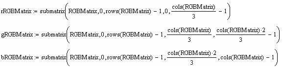
We obtain matrices describing the components of the model (R, G, B):
Calculate the Y-component of the YUV model:

The translation coefficients (they are constant and are determined by the peculiarities of human perception, and it is from a human position that we estimate the boundaries here):

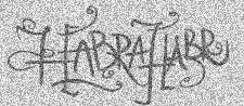
Result of conversion:
To suppress noise, use a blurred image filter Gauss.
Gauss function for the two-dimensional case:

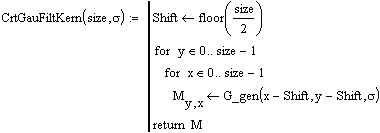
The method that makes up the filter core of size with parameter σ :
The procedure for applying a filter with a kernel of size and parameter σ to the matrix image Matrix :

You must select filter options that provide the best noise reduction. The influence of pixels on each other in Gaussian filtering is inversely proportional to the square of the distance between them: the proportionality coefficient, and, consequently, the degree of blurring, is determined by the parameter σ . An excessive increase in the coefficient will lead to an increase in averaging up to uniformly black color of all pixels:
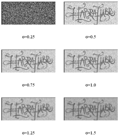
Choose σ = 1.0.
The filter core decreases to zero very quickly with distance from the point (0, 0), and therefore, in practice, we can limit ourselves to a convolution with a small window around (0, 0) (for example, following the three sigma rule, take a window radius of 3σ). Below is the result of applying a filter with a fixed value of the parameter σ , and a different size of the kernel (with the size parameter).
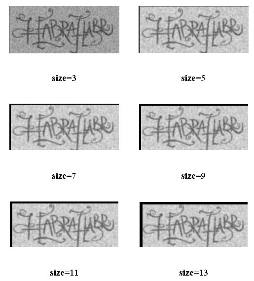
Choose size = 7. The result of applying the filter with the selected parameters is shown in the figure above.
The Sobel operator is often used in border detection algorithms. In fact, it is a discrete differential operator that calculates an approximate value of the image brightness gradient. The result of applying the Sobel operator at each point of the image is either the vector of the brightness gradient at that point, or its norm. The Sobel operator is based on the convolution of an image with small integer filters in the vertical and horizontal directions, so it is relatively easy to calculate it. On the other hand, the approximation of the gradient used by him is rather rough, this especially affects the high-frequency oscillations of the image.
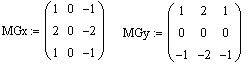
Filter cores:
Implementation (matches each point of the gradient vector):

The angle of the vector is quantized at 45 ° — such values are necessary for one of the following steps.
The figure below shows the result of applying the operator to the blurred (A) and original (in grayscale) image (B).

Boundary pixels are declared pixels in which a local gradient maximum is reached in the direction of the gradient vector. The direction must be a multiple of 45 °.
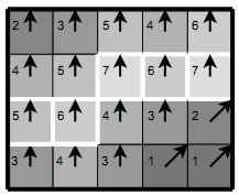
The principle of suppression is illustrated in the figure above. Almost all the pixels in the example are “oriented upwards,” so the gradient value at these points will be compared with the lower and upstream pixels. The white outlined pixels will remain in the resulting image, the rest will be suppressed.
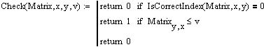
The implementation of checking the point of belonging to the image:

Value Comparison:
Implement suppression:
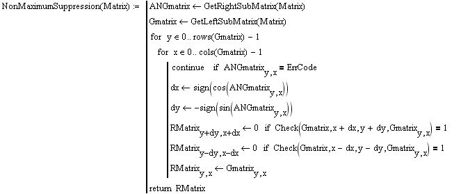
After the suppression of non-highs, the edges became more accurate and thin.
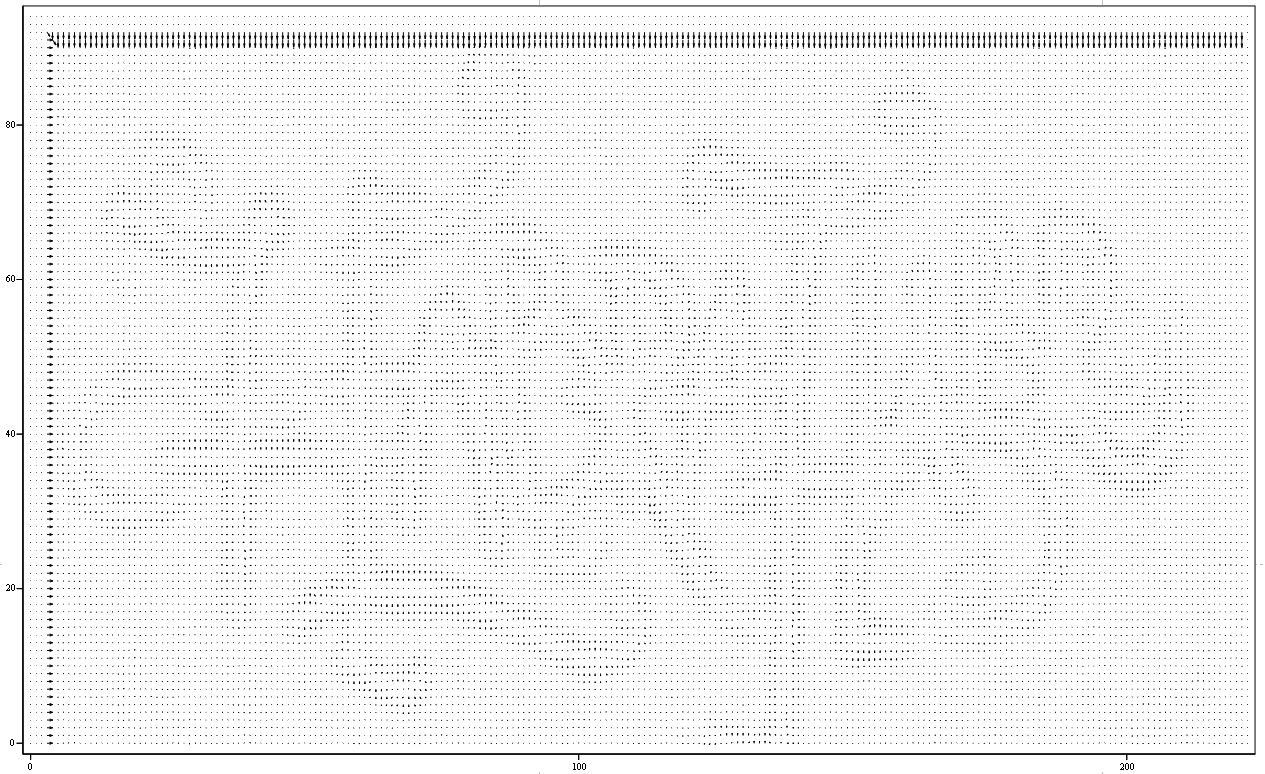
Below, in the first figure, the vector field of gradients (angles are multiples of 45 °) of the entire original (that is, before the suppression) image is presented, and in the second - a small fragment.

The next step is to use a threshold to determine whether or not the border is at a given point in the image. The smaller the threshold, the more borders there will be, but the more susceptible to noise the result will be, highlighting the extra image data. Conversely, a high threshold can ignore weak edges or get a border in fragments.
Canny border selection uses two filtering thresholds: if a pixel value is higher than the upper limit, it takes the maximum value (the border is considered reliable), if lower, the pixel is suppressed, points with a value falling in the range between the thresholds take a fixed average value (they will be refined by next stage).
Implementation:

The result of application with thresholds of 55% and 60% of the range is shown in the figure below.
Simplified, the task is reduced to the selection of groups of pixels that received an intermediate value at the previous stage and to assign them to the border (if they are connected to one of the established borders) or to suppress them (otherwise). A pixel is added to a group if it touches it in one of 8 directions.
Implementation:

Trace result:

In the development process, I used the following sources (mainly [1]):
I will be glad to criticism and comments, as the field of computer vision is not related to my professional activity.
upd And here is the criticism. Thanks to Andreyivanoff for pointing out fundamental errors in the algorithm and the link to the article ( here ).
upd2 andreyivanoff gives important comments on the algorithm here .
Recently, on Habré, Kanni’s border selection algorithm (which, to my surprise, translates literally: tricky) has often been mentioned. So, I matured to share with the public my experience in implementing this detector.
In my spare time, in order to educate myself, I study algorithms (including machine vision). I deal with this unprofessionally, in many respects adhering to popular scientific literature or my own algorithmic solutions.
On the one hand, to simplify coding, and on the other hand, to give a narration to a note of brainfuck programming, I will show implementation in the Mathcad computer algebra environment (algorithms tested in versions 13 and 14), with as little as possible using specific built-in methods. Such a campaign, in my opinion, improves the perception of the demonstration, and facilitates the possible transfer of algorithms to other design / development environments. It should be noted that some stages of the Kanni detector operation may involve not only various optimization (for example, software implementation of the Sobel operator using SIMD-expansion of the processor command system), but also the possibility of replacing some operators (methods) with others (for example, the Sobel operator can be replaced operator Roberts or Pruitt), and the possibility of varying the coefficients that define the parameters of the operators.
This version was created for reasons of maximum ease of implementation in the Mathcad environment, possibly at the expense of performance in terms of speed and quality of detection, and is presented as a demonstration of the main stages of the functioning of the Canny detector.
Highlighting Kanni Borders
Kanni (John F. Canny; 1953) studied the mathematical problem of obtaining a filter that is optimal according to the criteria for isolating, localizing and minimizing several responses of one edge. This means that the detector should react to the borders, but at the same time ignore the false ones, accurately determine the border line (without fragmenting it) and respond to each border once, thus avoiding the perception of wide bands of brightness as a combination of borders. Kanni introduced the concept of Non-Maximum Suppression, which means that the pixels at the edges are declared at which the local maximum of the gradient in the direction of the gradient vector is reached.
Although his work was carried out at the dawn of computer vision (1986), Kanney's boundary detector is still one of the best detectors. In addition to particular special cases, it is difficult to find a detector that would work substantially better than the Kanni detector.
')
Task
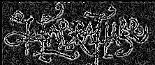
As a demonstration of the operation of the algorithm, the problem of boundary selection in the next image will be solved.
The algorithm consists of five separate steps:
- Smoothing Blur image to remove noise.
- Search for gradients . Borders are marked where the gradient of the image acquires the maximum value.
- Suppression of non-highs . Only local maxima are marked as boundaries.
- Dual threshold filtering . Potential boundaries are determined by thresholds.
- Trace area of ambiguity . The resulting boundaries are determined by suppressing all edges that are not bound to certain (strong) boundaries.
Conversion to grayscale
To convert the original image into an image in grayscale, you need to get its "brightness" -component. For this, it is convenient to present the image in the YUV color model (or HSL, HSV, others).
Initially, the picture is presented in the RGB color model, and the load function returns three components in the form of a single matrix.
To transfer the image to the YUV model, perform the following operations.
We obtain matrices describing the components of the model (R, G, B):
Calculate the Y-component of the YUV model:
The translation coefficients (they are constant and are determined by the peculiarities of human perception, and it is from a human position that we estimate the boundaries here):
Result of conversion:
Smoothing
To suppress noise, use a blurred image filter Gauss.
Gauss function for the two-dimensional case:
The method that makes up the filter core of size with parameter σ :
The procedure for applying a filter with a kernel of size and parameter σ to the matrix image Matrix :
You must select filter options that provide the best noise reduction. The influence of pixels on each other in Gaussian filtering is inversely proportional to the square of the distance between them: the proportionality coefficient, and, consequently, the degree of blurring, is determined by the parameter σ . An excessive increase in the coefficient will lead to an increase in averaging up to uniformly black color of all pixels:
Choose σ = 1.0.
The filter core decreases to zero very quickly with distance from the point (0, 0), and therefore, in practice, we can limit ourselves to a convolution with a small window around (0, 0) (for example, following the three sigma rule, take a window radius of 3σ). Below is the result of applying a filter with a fixed value of the parameter σ , and a different size of the kernel (with the size parameter).
Choose size = 7. The result of applying the filter with the selected parameters is shown in the figure above.
Gradient Search
The Sobel operator is often used in border detection algorithms. In fact, it is a discrete differential operator that calculates an approximate value of the image brightness gradient. The result of applying the Sobel operator at each point of the image is either the vector of the brightness gradient at that point, or its norm. The Sobel operator is based on the convolution of an image with small integer filters in the vertical and horizontal directions, so it is relatively easy to calculate it. On the other hand, the approximation of the gradient used by him is rather rough, this especially affects the high-frequency oscillations of the image.
Filter cores:
Implementation (matches each point of the gradient vector):
The angle of the vector is quantized at 45 ° — such values are necessary for one of the following steps.
The figure below shows the result of applying the operator to the blurred (A) and original (in grayscale) image (B).
Suppress non-highs
Boundary pixels are declared pixels in which a local gradient maximum is reached in the direction of the gradient vector. The direction must be a multiple of 45 °.
The principle of suppression is illustrated in the figure above. Almost all the pixels in the example are “oriented upwards,” so the gradient value at these points will be compared with the lower and upstream pixels. The white outlined pixels will remain in the resulting image, the rest will be suppressed.
The implementation of checking the point of belonging to the image:
Value Comparison:
Implement suppression:
After the suppression of non-highs, the edges became more accurate and thin.
Below, in the first figure, the vector field of gradients (angles are multiples of 45 °) of the entire original (that is, before the suppression) image is presented, and in the second - a small fragment.
Dual threshold filtering
The next step is to use a threshold to determine whether or not the border is at a given point in the image. The smaller the threshold, the more borders there will be, but the more susceptible to noise the result will be, highlighting the extra image data. Conversely, a high threshold can ignore weak edges or get a border in fragments.
Canny border selection uses two filtering thresholds: if a pixel value is higher than the upper limit, it takes the maximum value (the border is considered reliable), if lower, the pixel is suppressed, points with a value falling in the range between the thresholds take a fixed average value (they will be refined by next stage).
Implementation:
The result of application with thresholds of 55% and 60% of the range is shown in the figure below.
Trace ambiguity
Simplified, the task is reduced to the selection of groups of pixels that received an intermediate value at the previous stage and to assign them to the border (if they are connected to one of the established borders) or to suppress them (otherwise). A pixel is added to a group if it touches it in one of 8 directions.
Implementation:
Trace result:
List of sources
In the development process, I used the following sources (mainly [1]):
- Canny Edge Detection www.cvmt.dk/education/teaching/f09/VGIS8/AIP
- Wikipedia Edge detection en.wikipedia.org/wiki/Edge_detection
- Wikipedia Sobel operator ru.wikipedia.org/wiki/Soobel_ operator
- Algorithmic bases of raster graphics www.intuit.ru/department/graphics/rastrgraph/8/rastrgraph_8.html
I will be glad to criticism and comments, as the field of computer vision is not related to my professional activity.
upd And here is the criticism. Thanks to Andreyivanoff for pointing out fundamental errors in the algorithm and the link to the article ( here ).
upd2 andreyivanoff gives important comments on the algorithm here .
Source: https://habr.com/ru/post/114589/
All Articles