About image gradient

annotation

The article describes the calculation of the gradient in the image using differential patterns. An obvious and beautiful way to optimize the sequence is proposed: “Lubrication -> Gradient Calculation”. The article is a necessary preamble to the planned article on fast and cunning algorithms for the selection of contours and angles.

Introduction

Gradient is a vector quantity that indicates the direction of the fastest increase of a certain quantity. In our case, “some value” is a two-dimensional function of image brightness, let us assume that we are considering a “pseudo-continuous” image, then the gradient vector is defined by the formula

where I is our image.
In practice, the picture is discrete and in the classical sense, the derivative does not exist; therefore, its difference analogs are used, for example, in the simplest case

- left differential derivative. There are a great many difference analogs, and they all have different approximation orders, more details here . An increase in the approximation order, for example, as here in the theory should lead to an increase in the accuracy of the derivative calculation. Moreover, by increasing the number of elements in the approximation, we can increase the resistance to noise.
For example, we will use the difference analog of the first derivative, the sixth order of accuracy of the approximation in the discretization step:

Now suppose that I (i, j) are independent random variables distributed according to any law of distribution, and see the variances:

1. For the first approximation, we obtain:
2. For the second approximation, we obtain

As a rule, the dispersion of additive noise can be considered isotropic, and then the relations


Thus, the noise gain factor (1.17), in the case of approximation by a derivative of a higher order difference, is less than coefficient (2) in the case of approximation by a derivative by the left difference. It is logical that this greatly increases the computational cost. And now pictures:

Figure 1 - Original image , 2 - modulus of the gradient according to the first formula , 3 - modulus of the gradient according to the second formula.

')
As a result, we calculated the gradient, in which the noise component did not increase by 2 times but only 1.17 times, but again, if there is noise in the picture, then it would be nice to reduce its dispersion before (before calculating the gradient) - for example, blur the original image I , that is, to make a convolution for example with a Gaussian core f . Then the gradient is written as:

However, the following formula is known from the properties of the convolution operator:


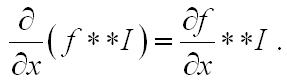
We calculate the derivative not by the image, but by the kernel f ; and the choice of the exact template for calculating the differential analogue of the derivative is limited only by the window size.

Thus, it is possible to construct the “Smaz - Gradient Calculation” algorithm:

1. We calculate the difference analogs of derivatives by the kernel,
2. We turn off the resulting kernel with the image
3. As a result, we obtain the components of the gradient vector.

In computational terms:
It was: One convolution with a window (NxN) for blurring, + two convolutions with specific windows (1xN, Nx1) for calculating derivatives.
It became: Two convolutions with specific windows (but now NxN) for calculating derivatives.
Calculating the gradient of a blurred image is a task that is very often encountered, for example, in sly detectors of angles and contours, which will be discussed next.

What will work faster, and most importantly - more resistant to noise? I propose to answer this question in the comments on the article by the readers themselves.