Algorithms for image contour selection
In the light of recent articles on image processing, I would like to talk a little about contour extraction algorithms: Roberts, Prewitt and Sobel methods (these methods are taken for consideration as the most well-known and frequently used).
I will not bother with volume theory, but I will confine myself to the minimum information necessary for understanding the essence of algorithms.
All of these methods are based on one of the basic properties of the brightness signal - discontinuity . The most common way to search for gaps is to process an image using a sliding mask , also called a filter, core, window, or pattern , which is a kind of square matrix corresponding to a specified group of pixels of the original image. Matrix elements are called coefficients . Handling such a matrix in any local transformations is called filtering or spatial filtering .
The spatial filtering scheme is illustrated in the figure below (see Figure 1).
')
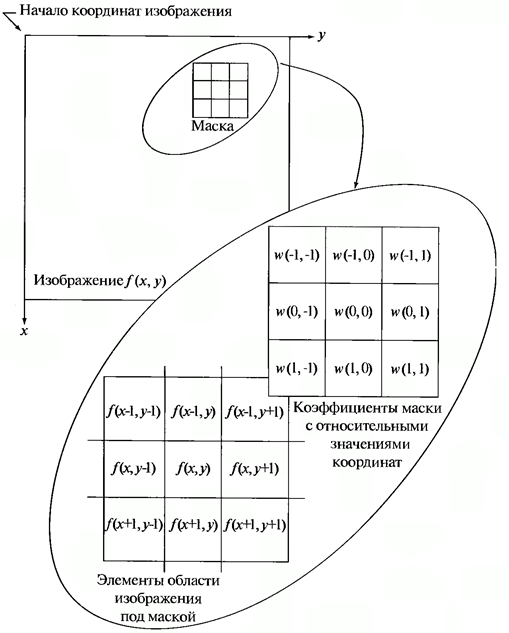
Figure 1. Spatial filtering scheme
The process is based on simply moving the filter mask from point to point in the image; at each point (x, y), the filter response is calculated using pre-defined links. In the case of linear spatial filtering, the response is given by the sum of the product of the filter coefficients and the corresponding pixel values in the area covered by the filter mask. For a 3x3 mask element shown in Figure 1, the result (response) R of the linear filtering at the point (x, y) of the image will be:
 (1.1)
(1.1)
that, as can be seen, is the sum of the products of the mask coefficients by the pixel values directly under the mask. In particular, we note that the coefficient w (0, 0) stands at f (x, y) , indicating that the mask is centered at the point (x, y) .
When detecting differences in brightness, discrete analogs of first and second order derivatives are used. For simplicity, one-dimensional derivatives will be considered.
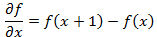
The first derivative of the one-dimensional function f (x) is defined as the difference of the values of neighboring elements:
 (1.2)
(1.2)
Here, the record is used in the form of a partial derivative in order to preserve the same notation in the case of two variables f (x, y) , where it is necessary to deal with partial derivatives along two spatial axes. The use of the partial derivative does not change the substance of the consideration.
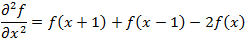
Similarly, the second derivative is defined as the difference of the neighboring values of the first derivative:
 (1.3)
(1.3)
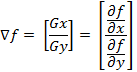
The calculation of the first derivative of a digital image is based on various discrete approximations of a two-dimensional gradient. By definition, the image gradient f (x, y) at the point (x, y) is a vector [2]:
 (1.4)
(1.4)
As is known from the course of mathematical analysis, the direction of the gradient vector coincides with the direction of the maximum rate of change of the function f at the point (x, y) [2].
An important role in the detection of contours is played by the modulus of this vector, which is denoted by ∇f and is equal to
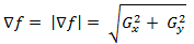 (1.5)
(1.5)
This value is equal to the value of the maximum rate of change of the function f at the point (x, y) , and the maximum is reached in the direction of the vector ∇f . The value of ∇f is also often called the gradient.
The direction of the gradient vector is also an important characteristic. Let α (x, y) be the angle between the direction of the vector ∇f at the point (x, y) and the x axis. As is known from mathematical analysis [2],
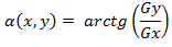 (1.6)
(1.6)
From here it is easy to find the direction of the contour at the point (x, y) , which is perpendicular to the direction of the gradient vector at that point. And you can calculate the image gradient by calculating the partial derivatives f / ∂x and ∂f / ∂y for each point.
Let the 3x3 area shown in the figure below (see Fig. 2) be the brightness values in the neighborhood of some image element.
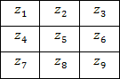
Figure 2. The neighborhood 3x3 inside the image
One of the easiest ways to find the first partial derivatives at consists in applying the following cross gradient Roberts operator [1]:
 (1.7)
(1.7)
and
 (1.8)
(1.8)
These derivatives can be implemented by processing the entire image using the operator, described by masks in Figure 3, using the filtering procedure described earlier.
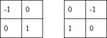
Figure 3. Roberts operator masks
The implementation of masks with dimensions of 2x2 is not very convenient, since they have no clearly defined central element, which significantly affects the result of filtering. But this “minus” generates a very useful feature of this algorithm - high speed image processing.
The Prewitt operator, as well as the Roberts operator, operates on the 3x3 image area shown in Figure 2, only the use of such a mask is given by other expressions:
 (1.9)
(1.9)
and
 (1.10)
In these formulas, the difference between the sums in the upper and lower rows of a 3x3 neighborhood is an approximate value of the derivative along the x axis, and the difference between the sums along the first and last columns of this neighborhood is the derivative along the y axis. To implement these formulas, use the operator described by the masks in Figure 4, which is called the Prewitt operator.
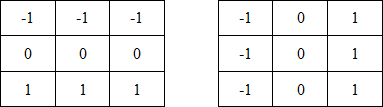
Figure 4. Prewitt operator masks
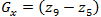
The Sobel operator also uses the 3x3 image area shown in Figure 2. It is quite similar to the Prewitt operator, and the modification is to use the weighting factor 2 for the middle elements:
 (1.11)
and
 (1.12)
This increased value is used to reduce the smoothing effect by adding more weight to the midpoints.
The masks used by the Sobel operator are shown in the figure below (see Fig. 5).
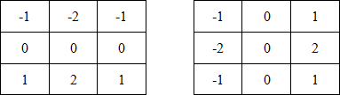
Figure 5. Sobel operator masks
The masks discussed above are used to obtain the components of the gradient . To calculate the magnitude of the gradient, these components must be used together:
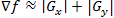 (1.14)
or
 (1.15)
Well, in the end I will demonstrate the results of image processing (see Figures 6-8) by the described methods.
Figure 6. Original image №1
Figure 7. The original image number 2
Figure 8. Original image №3
The results of the processing by the methods of Roberts, Prewitt and Sobel are shown below:
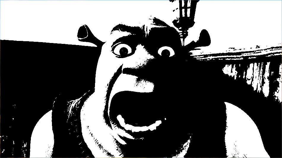
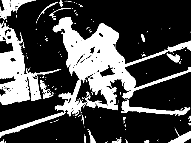
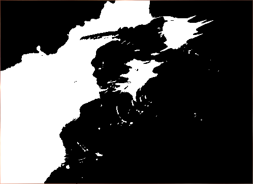
Figure 9. Original images after Roberts processing
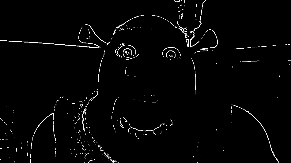

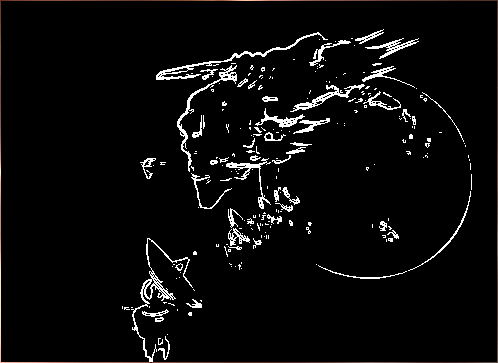
Figure 10 . Original images after processing by Prewitt
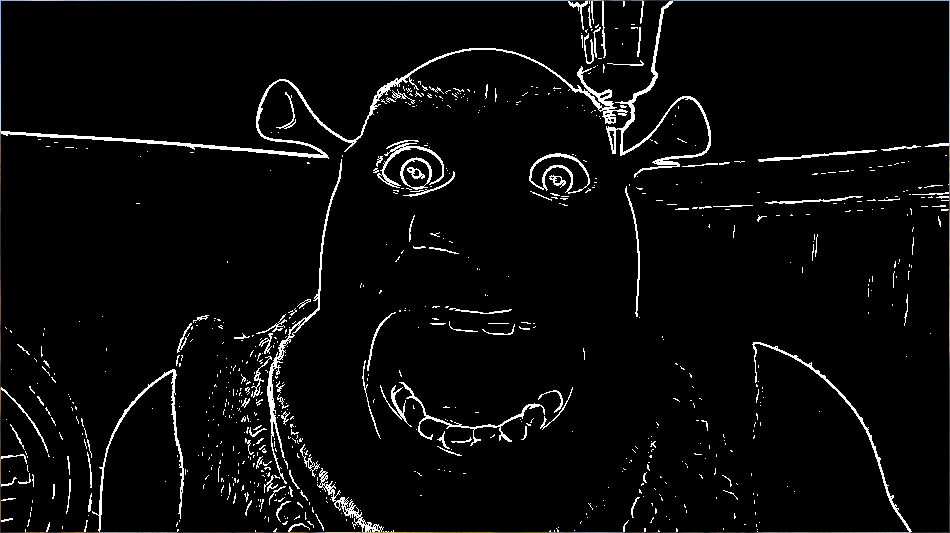
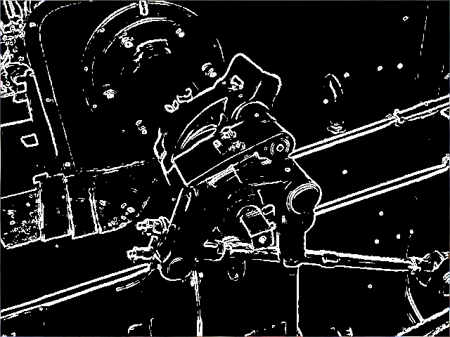
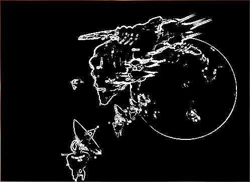
Figure 11. Source images after Sobel processing
I will not bother with volume theory, but I will confine myself to the minimum information necessary for understanding the essence of algorithms.
All of these methods are based on one of the basic properties of the brightness signal - discontinuity . The most common way to search for gaps is to process an image using a sliding mask , also called a filter, core, window, or pattern , which is a kind of square matrix corresponding to a specified group of pixels of the original image. Matrix elements are called coefficients . Handling such a matrix in any local transformations is called filtering or spatial filtering .
The spatial filtering scheme is illustrated in the figure below (see Figure 1).
')
Figure 1. Spatial filtering scheme
The process is based on simply moving the filter mask from point to point in the image; at each point (x, y), the filter response is calculated using pre-defined links. In the case of linear spatial filtering, the response is given by the sum of the product of the filter coefficients and the corresponding pixel values in the area covered by the filter mask. For a 3x3 mask element shown in Figure 1, the result (response) R of the linear filtering at the point (x, y) of the image will be:
(1.1)that, as can be seen, is the sum of the products of the mask coefficients by the pixel values directly under the mask. In particular, we note that the coefficient w (0, 0) stands at f (x, y) , indicating that the mask is centered at the point (x, y) .
When detecting differences in brightness, discrete analogs of first and second order derivatives are used. For simplicity, one-dimensional derivatives will be considered.
The first derivative of the one-dimensional function f (x) is defined as the difference of the values of neighboring elements:
(1.2)Here, the record is used in the form of a partial derivative in order to preserve the same notation in the case of two variables f (x, y) , where it is necessary to deal with partial derivatives along two spatial axes. The use of the partial derivative does not change the substance of the consideration.
Similarly, the second derivative is defined as the difference of the neighboring values of the first derivative:
(1.3)The calculation of the first derivative of a digital image is based on various discrete approximations of a two-dimensional gradient. By definition, the image gradient f (x, y) at the point (x, y) is a vector [2]:
(1.4)As is known from the course of mathematical analysis, the direction of the gradient vector coincides with the direction of the maximum rate of change of the function f at the point (x, y) [2].
An important role in the detection of contours is played by the modulus of this vector, which is denoted by ∇f and is equal to
(1.5)This value is equal to the value of the maximum rate of change of the function f at the point (x, y) , and the maximum is reached in the direction of the vector ∇f . The value of ∇f is also often called the gradient.
The direction of the gradient vector is also an important characteristic. Let α (x, y) be the angle between the direction of the vector ∇f at the point (x, y) and the x axis. As is known from mathematical analysis [2],
(1.6)From here it is easy to find the direction of the contour at the point (x, y) , which is perpendicular to the direction of the gradient vector at that point. And you can calculate the image gradient by calculating the partial derivatives f / ∂x and ∂f / ∂y for each point.
Roberts operator
Let the 3x3 area shown in the figure below (see Fig. 2) be the brightness values in the neighborhood of some image element.
Figure 2. The neighborhood 3x3 inside the image
One of the easiest ways to find the first partial derivatives at
consists in applying the following cross gradient Roberts operator [1]: (1.7)and
(1.8)These derivatives can be implemented by processing the entire image using the operator, described by masks in Figure 3, using the filtering procedure described earlier.
Figure 3. Roberts operator masks
The implementation of masks with dimensions of 2x2 is not very convenient, since they have no clearly defined central element, which significantly affects the result of filtering. But this “minus” generates a very useful feature of this algorithm - high speed image processing.
Operator Prewitt
The Prewitt operator, as well as the Roberts operator, operates on the 3x3 image area shown in Figure 2, only the use of such a mask is given by other expressions:
(1.9)and
(1.10)In these formulas, the difference between the sums in the upper and lower rows of a 3x3 neighborhood is an approximate value of the derivative along the x axis, and the difference between the sums along the first and last columns of this neighborhood is the derivative along the y axis. To implement these formulas, use the operator described by the masks in Figure 4, which is called the Prewitt operator.
Figure 4. Prewitt operator masks
Sobel operator
The Sobel operator also uses the 3x3 image area shown in Figure 2. It is quite similar to the Prewitt operator, and the modification is to use the weighting factor 2 for the middle elements:
(1.11)and
(1.12)This increased value is used to reduce the smoothing effect by adding more weight to the midpoints.
The masks used by the Sobel operator are shown in the figure below (see Fig. 5).
Figure 5. Sobel operator masks
The masks discussed above are used to obtain the components of the gradient
. To calculate the magnitude of the gradient, these components must be used together: (1.14)or
(1.15)Well, in the end I will demonstrate the results of image processing (see Figures 6-8) by the described methods.
Figure 6. Original image №1
Figure 7. The original image number 2
Figure 8. Original image №3
The results of the processing by the methods of Roberts, Prewitt and Sobel are shown below:
Figure 9. Original images after Roberts processing
Figure 10 . Original images after processing by Prewitt
Figure 11. Source images after Sobel processing
Bibliography
- R. Gonzalez, R. Woods Digital Image Processing - M: Technosphere, 2005 - 1007s
- Kudryavtsev L.V. A short course of mathematical analysis - M .: Science, 1989 - 736s
- Anisimov B.V. Recognition and digital image processing - M .: Higher. School, 1983 - 295s
Source: https://habr.com/ru/post/114452/
All Articles