Quantile Image Segmentation

Segmentation is the assignment of tags to image pixels so that areas with similar properties in a certain sense have the same labels. Also, segmentation is sometimes called the search for the projection of an object in an image. This topic will tell you about a simple but effective method of searching for the projection of an object, called the quantile method. The area of ​​applicability of the method is indicated and some modifications that increase the efficiency are given.

Some concepts and assumptions

In order to be able to find an object in an image, we must assume that the object has some distinctive features represented in the image. As such a feature, we will use the brightness. We call an object a bright spot if the average brightness of the pixels belonging to the projection of the object is higher than the average brightness of the pixels of the surrounding background. (Dark spots are determined in a similar way.) Such objects are found, for example, in infrared aerial photographs of a terrain: a heated technique looks brighter than the surrounding earth. In general, the practice (mainly in the military) shows that in many cases it is possible to select such a range of wavelengths for shooting, so that the condition of the difference in average brightness is fulfilled.

Segmentation of the entire image is a difficult task at once, so it is often broken down into subtasks: first, small fragments are found in the image that presumably contain the object of interest, and then they are segmented. A small (usually, without loss of generality, square) image fragment containing only the object itself and some of its surroundings (background) is called the zone of interest . In our case, we will work with the zones of interest. The first subtask (search for zones of interest) is solved by its own methods and is not discussed in this topic.
')
It is also assumed that we know the geometric features of the object, namely, the area of ​​the projection of the object in the image. This assumption is fulfilled when we know in advance what we are looking for in the image, but we do not know where the object is located. It is also assumed that the projection of the object is a connected set .

Initial data and problem statement

So, we have an image of the zone of interest, on which the object is located, which is a bright spot. In reality, images are not perfect, many random factors impede the segmentation task. Therefore, the original image is distorted by Gaussian noise (in connection with the presence of noise, we talked about medium brightness, and not just brightness, in the definition of a bright spot). We know the area S of the projection of the object in the image.

It is necessary to mark the pixels belonging to the projection of the object.

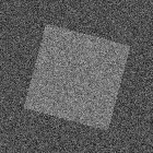
As an example, take this image:

It has a size of 140x140 pixels. It shows a square of 80x80 pixels, located in the center and rotated 15 degrees. The average background brightness is 80, the average brightness of the object is 120. Gaussian noise has a standard deviation of 20.

Original Quantile Method

The quantile method was first described in [1]. The method in its original form assumes that the brightness of any pixel of the object in the image is higher than the brightness of any pixel of the background. From this assumption follows a simple segmentation method. Sort all the pixels of the image in descending order of brightness. From our assumption it follows that the pixels belonging to the projection of the object will be located at the beginning of the ordered sequence. Therefore, we can mark the first S pixels with the label “Object” - they will belong to the desired projection.

Unfortunately, this assumption is not always fulfilled. Our picture here is also no exception. The result of the segmentation method described below. Object pixels are marked in white, background pixels are black.


It is worth discussing another small issue. On real images, like ours, it is unlikely that it will be possible to pick up such a threshold brightness value, so that the greater threshold has exactly S pixels of the image. Often at one threshold of brightness (t) we cut off A <S pixels, and at threshold (t-1) - B> S pixels. “Arrange”, as suggested above, the pixels of the same brightness, we can not, we must either take all the pixels of brightness (t), or not take. The easiest way to decide is to see what is less: (SA) or (BS). We look at which number - A or B - is closer to what needs to be obtained, and take the corresponding threshold. This method was used to obtain images presented in the topic.

"Improved" quantile method

The assumption of the original method is often not carried out due to the influence of noise: although on average the brightness of an object pixel is higher than the brightness of the background pixel, but in some cases it can be the other way around. (It is worth noting here that when the difference in average brightness is large and the noise dispersion is small, the first method can also work.) The “improved” quantile method uses precisely the assumption about the difference in average values ​​of object and background brightness.

Mathematical statistics tells us that in our case of Gaussian noise, the estimate of the average brightness value at a point, made by calculating the average arithmetic brightness over a neighborhood, will be a consistent and unbiased estimate. In other words, we do not know the true average brightness for each pixel of the image, but we can take some neighborhood of this pixel B (z, r), where z is the coordinates of the pixel, r is the radius of the neighborhood:

and calculate the arithmetic average of the brightness for this neighborhood:

Here Q is the set of image pixels, x _t is the brightness of the image at t. We can quite legally use this estimate instead of the true average value, and the larger the radius of the neighborhood we take, the more accurate the estimate will be.

In the “improved” quantile method, first of all, the arithmetic average is calculated using the above formula at each point. Then the same procedure is performed as in the original method, but instead of the immediate brightness values, the mean values ​​are used. (Note: instead of smoothing the image by calculating the arithmetic average, in practice, Gaussian image smoothing is often used - this is a weighted average with coefficients of the corresponding distribution; such smoothing solves some problems of the arithmetic average.)

For our image we get the following result (segmentation with r = 1):

The result has noticeably improved. Increase the radius to calculate the arithmetic average to r = 2:

With a radius of 2 extraneous "specks" completely gone! It can be noted, however, that with increasing radius, the boundary of the object is distorted. This is due to the fact that the estimate of the true average of the arithmetic average is true only when the neighborhood B (z, r) lies either entirely on the object, or entirely on the background, that is, when random variables with the same estimated average fall into it by value. On the border, pixels and background and object fall into the neighborhood, which naturally distorts the estimate.

Algorithm modification

As stated above, it is assumed that the projection of the object is a connected set. In this regard, we can filter out the extra “spots” that arise after segmentation as follows: we calculate the area of ​​each connected component and leave the one of them, the area of ​​which is the largest.

Below are the results obtained after the selection of the largest connected component on the images with the segmentation result by the original method and the “improved” method with r = 1 (with r = 2, only one connected component remains):

In both cases, this made it possible to filter out extra “spots” and get a good result even for the original quantile method.

Conclusion

The quantile method was invented long ago, very simple to implement. For all its simplicity, the method gives good results. Although in the currently complex image processing tasks, such simple methods are not enough to get the desired result and more complex segmentation methods have been developed, simple methods do not lose their relevance. They are used as an integral part of more complex algorithms, and are also very useful for implementing “in hardware”, when simple, in terms of calculations, but reliable algorithms are required.

Sources

[1] Doyle W. Operations useful for invariant pattern recognition. // Journal ACM. 1962. Vol. 9, No. 2. P. 259-267.